Introduction to the bioinformatic analysis of eDNA metabarcoding data

Overview

Teaching: 15 min
Exercises: 0 min

Questions

• What are the main components of metabarcoding pipelines?

Objectives

• Review typical metabarcoding workflows

eDNA Workshop

Welcome to the environmental DNA (eDNA) workshop session of the Otago Bioinformatic Spring School 2022!

The primary goal of this course is to introduce you to the analysis of metabarcoding sequence data, with a specific focus on environmental DNA or eDNA, and make you comfortable to explore your own next-generation sequencing data. During this course, we’ll introduce the concept of metabarcoding and go through the different steps of a bioinformatic pipeline, from raw sequencing data to a frequency table with taxonomic assignments. At the end of this course, we hope you will be able to assemble paired-end sequences, demultiplex fastq sequencing files, filter sequences based on quality, cluster and denoise sequence data, build your own custom reference database, assign taxonomy to OTUs, and analyse the data in a statistically correct way.

Introduction

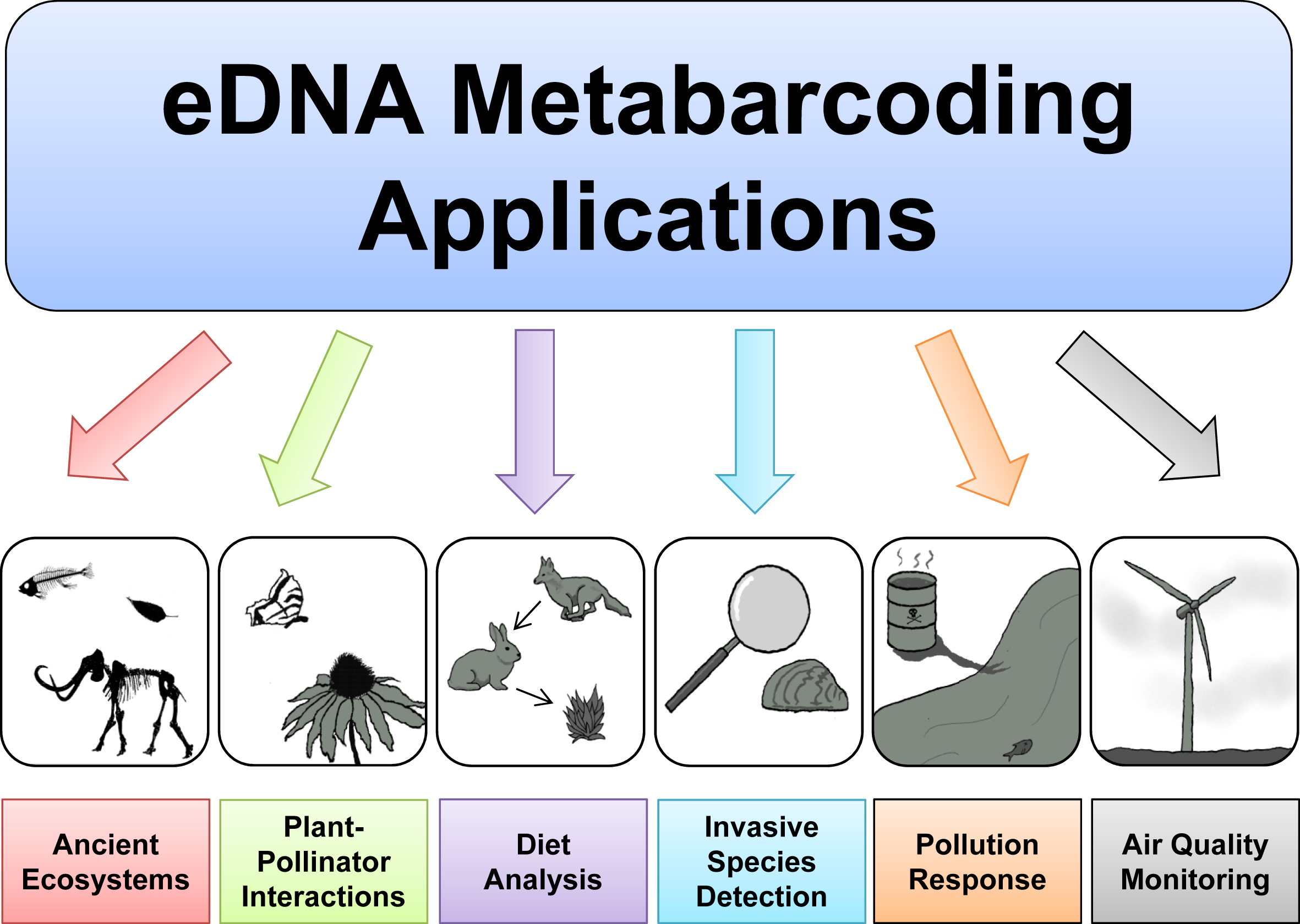
Based on the 3 excellent presentations at the start of today’s workshop, we can get an understanding of how broadly applicable eDNA metabarcoding is and how many many research fields are using this technology to answer questions about biological systems.

Before we get started with coding, we will first introduce the data we will be analysing today, some of the software programs available (including the ones we will use today), and the general structure of a bioinformatic pipeline to process metabarcoding data. Finally, we’ll go over the folder structure we suggest you use during the bioinformatic processing of metabarcoding data to help keep an overview of what is going on and ensure reproducibility of the bioinformatic pipeline.

Experimental setup

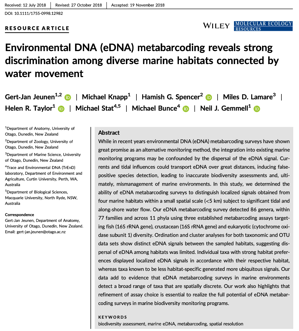
The data we will be analysing today is taken from an experiment we published in 2018 in Molecular Ecology Resources, where we wanted to determine the spatial resolution of aquatic eDNA in the marine environment. To investigate the spatial resolution, we visited a marine environment with high dynamic water movement where we knew from traditional monitoring that there were multiple habitats present on a small spatial scale containing different community assemblages. Our hypothesis was as follows, if the spatial resolution of aquatic eDNA is high, we would encounter distinct eDNA signals at each habitat resembling the residing community. However, if aquatic eDNA is transported through water movement, from currents and tidal waves, similar eDNA signals would be obtained across this small sampling area, which would be indicative of a low spatial resolution for aquatic eDNA. Our experiment consisted of five replicate water samples (2l) at each sampling point. Water was filtered using a vacuum pump and extracted using a standard Qiagen DNeasy Blood & Tissue Kit. All samples were amplified using three metabarcoding primer sets to target fish and crustacean diversity, specifically. We also used a generic COI primer set to amplify eukaryotic eDNA signals.

For today’s data analysis, we subsetted the data to only include two sampling sites and we’ll only be looking at the fish sequencing data. The reason for doing so, is to ensure all bioinformatic steps will take maximum a couple of minutes, rather than hours or days to complete the full analysis.

Software programs used for eDNA metabarcoding

Due to the popularity of metabarcoding, a myriad of software packages and pipelines are currently available. Furthermore, software packages are continuously updated with new features, as well as novel software programs being designed and published. We will be using several software programs during today’s workshop, however, we would like to stress that the pipeline used in the workshop is by no means better than other pipelines and we urge you to explore alternative software programs and trial them with your own data after this workshop.

Two notes of caution about software programs:

1. While some software programs are only able to complete a specific aspect of the bioinformatic pipeline, others are able to handle all steps. It might therefore seem easier to use a program that can be used to run through the pipeline in one go. However, this could lead to a ‘black box’ situation and can limit you when other software programs might have additional options or better alternatives. It is, therefore, recommended to understand each step in the bioinformatic pipeline and how different software programs implement these steps. Something we hope you will take away from today’s eDNA workshop.
2. One issue you will run into when implementing severl software programs in your bioinformatic pipeline is that each program might change the structure of the files in a specific manner. These modifications might lead to incompatability issues when switching fto the next program. It is, therefore, important to understand how a specific program changes the structure of the sequencing file and learn how these modification can be reverted back (through simple python or bash scripts). We will talk a little bit more about file structure and conversion throughout the workshop.

Below, we can find a list of some of the software programs that are available for analysing metabarcoding data (those marked with a ‘*’ will be covered in this workshop):

• Cutadapt* (webpage) is a program that find and removes adapter sequences, primers, and other types of unwated sequences from high-throughput sequencing reads. We will use this program to demultiplex our data.

• USEARCH/VSEARCH* (webpage), and the open-source version (which we will use) (VSEARCH*), has many utilities for running metabarcoding analyses. Many of the most common pipelines use at least some of the tools from these packages.

• CRABS* (webpage) is a software package developed by our team that lets you build and curate custom reference databases.

• Qiime2 is actually a collection of different programs and packages, all compiled into a single ecosystem so that all things can be worked together. On the Qiime2 webpage there is a wide range of tutorials and help.

• Dada2 is a good program, run in the R language. There is good documentation and tutorials for this on its webpage. You can actually run Dada2 within Qiime, but there are a few more options when running it alone in R.

• Mothur has long been a mainstay of metabarcoding analyses, and is worth a look

• Another major program for metabarcoding is OBITools, which was one of the first to specialise in non-bacterial metabarcoding datasets. The newer version, updated for Python 3, is currently in Beta. Check the main webpage to keep track of its development.

Additionally, there are several good R packages that can be used to analyse and graph results. Chief among these are Phyloseq and DECIPHER.

General overview of the bioinformatic pipeline

Although software options are numerous, each pipeline follows more or less the same basic steps and accomplishes these steps using similar tools. Before we get started with coding, let’s go quickly over the main steps of the pipeline to give you a clear overview of what we will cover today. For each of these steps, we will provide more information when we cover those sections during the workshop.

Prior to the general steps of the metabarcoding pipeline, you might need to conduct a few additional steps, depending on how the library was prepared for sequencing and how the library was sequenced:

• Merging of paired-end sequencing data: Your library can either be sequenced single-end or paired-end. If your library was sequenced single-end, the amplicons will be contained in a single Illumina read and the data will be provided in a single file, the R1 fastq file. If so, no additional step is needed. If your library was sequenced paired-end, on the other hand, you will have been given two files by the sequencing service, i.e., the R1 and R2 fastq files. If so, the amplicons are split into two parts and the R1 and R2 files will need to be merged prior to the bioinformatic pipeline. An example software package that can accomplish this is PEAR (webpage). Since the example sequencing data used during the workshop is single-end, we will not cover the merging of reads in detail.

• Demultiplexing of sequencing data: When you receive sequencing data from the sequencing service, the data can be split up into a single file per sample. If so, no additional step is needed. However, sometimes you receive only a single fastq file, with no information in the filename or sequence header name on which sequences belong to which sample. In this case, we will need to demultiplex the data, i.e., assigning sequences to samples by locating the forward and reverse barcode and identifying to which sample they belong. Demultiplexing the sample data is something we will cover during today’s workshop in one of the first sections.

Once you have a single fastq file for each sample, the bioinformatic pipeline follows these main steps:

1. Quality filtering: remove low quality sequences.
2. Dereplication: find all unique sequences in the data.
3. Chimera removal: discard chimeric sequences that were generated during PCR amplification.
4. Clustering or Denoising: retrieve all biologically meaningful sequences in the dataset.
5. OTU table generation: create an OTU table, similar to a frequency table in traditional ecology.
6. Taxonomic assignment: create a custom reference database and assign a taxonomic ID to each biologically meaningful sequence.

After all of these steps, you are ready to move forward with the statistical analysis of your data, using either R or python.

Using scripts to execute code

One final topic we need to cover before we get started with coding is the use of scripts to execute code. During this workshop, we will create very small and simple scripts that contain the code used to process the sequencing data. While it is possible to run the commands without using scripts, it is good practice to use this method for the following three reasons:

1. By using scripts to execute the code, there is a written record of how the data was processed. This will make it easier to remember how the data was processed in the future.
2. While the sample data provided in this tutorial is small and computing steps take up a maximum of several minutes, processing large data sets can be time consuming. It is, therefore, recommended to process a small portion of the data first to test the code, modify the filenames once everything is set up, and run it on the full data set.
3. Scripts can be reused in the future by changing file names, saving you time by not having to constantly write every line of code in the terminal. Minimising the amount needing to be written in the terminal will, also, minimise the risk of receiving error messages due to typo’s.

The folder structure

That is it for the intro, let’s get started with coding!

First, we’ll have a look at the folder structure we will be using during the workshop. For any project, it is important to organise your various files into subfolders. Through the course you will be navigating between folders to run your analyses. It may seem confusing or tedious, especially as there are only a few files. Remember that for many projects you can easily generate hundreds of files, so it is best to start with good practices from the beginning.

Let’s navigate to the edna folder in the ~/obss_2022/ directory. Running the ls -ltr command outputs the following subfolders:

• raw/
• input/
• output/
• meta/
• scripts/
• final/
• refdb/
• stats/

Most of these are currently empty, but by the end of the course they will be full of the results of your analysis.

So, let’s begin!

Key Points

• Most metabarcoding pipelines include the same basic components

• Frequency tables are key to metabarcoding analyses

Demultiplexing and Trimming

Overview

Teaching: 20 min
Exercises: 10 min

Questions

• What are the different primer design methods for metabarcoding?

• How do we demultiplex and quality control metabarcoding data?

Objectives

• Learn the different methods for QC of metabarcoding data

Initial processing of raw sequence data

Introduction

To start, let’s navigate to the raw sequencing file in the raw folder within the ~/obss_2021/edna/ directory and list the files in the subdirectory.

$ cd ~/obss_2021/edna/raw/
$ pwd

/home/username/obss_2022/edna/raw

$ ls -ltr

-rwxr-x---  1 gjeunen  staff  124306274 16 Nov 12:39 FTP103_S1_L001_R1_001.fastq.gz

From the output, we can see that we have a single fastq file, the R1_001.fastq.gz file, indicating that the library was sequenced single-end. Therefore, we do not need to merge or assemble paired reads (see Introduction for more information). From the output, we can also see that the sequencing file is currently zipped. This is done to reduce file sizes and facilitate file transfer between the sequencing service and the customer. Most software will be able to read and use zipped files, so there is no need to unzip the file now. However, always check if this is the case when using new software.

Quality control

The first thing we will do with our sequencing file is to look at the quality and make sure everything is according to the sequencing parameters that were chosen. The program we will be using for this is FastQC (EMP). However, since you’ve already encountered this software program, we’ll just focus on the output for now.

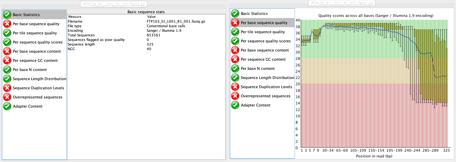
At this stage, we will be looking at the tabs Basic Statistics and Per base sequence quality. From this report, we can see that:

1. We have a total of 853,561 sequences.
2. The sequence length is 325 bp, identical to the cycle number of the specified sequencing kit.
3. Sequence quality is dropping significantly at the end, which is typical for Illumina sequencing data.

Demultiplexing sequencing data

Introduction to demultiplexing

Given that we only have a single sequence file containing all reads for multiple samples, the first step in our pipeline will be to assign each sequence to a sample, a process referred to as demultiplexing. To understand this step in the pipeline, we will need to provide some background on library preparation methods.

As of the time of writing this workshop, PCR amplification is the main method to generate eDNA metabarcoding libraries. To achieve species detection from environmental or bulk specimen samples, PCR amplification is carried out with primers designed to target a taxonomically informative marker within a taxonomic group. Furthermore, next generation sequencing data generates millions of sequences in a single sequencing run. Therefore, multiple samples can be combined. To achieve this, a unique sequence combination is added to the amplicons of each sample. This unique sequence combination is usually between 6 and 8 base pairs long and is referred to as ‘tag’, ‘index’, or ‘barcode’. Besides amplifying the DNA and adding the unique barcodes, sequencing primers and adapters need to be incorporated into the library to allow the DNA to be sequenced by the sequencing machine. How barcodes, sequencing primers, and adapters are added, and in which order they are added to your sequences will influence the data files you will receive from the sequencing service.

For example, traditionally prepared Illumina libraries (ligation and two-step PCR) are constructed in the following manner (the colours mentioned refer to the figure below):

1. Forward Illumina adapter (red)
2. Forward barcode sequence (darkgreen)
3. Forward Illumina sequencing primer (orange)
4. Amplicon (including primers)
5. Reverse Illumina sequencing primer (lightblue)
6. Reverse barcode sequence (lightgreen)
7. Reverse Illumina adapter (darkblue)

This construction allows the Illumina software to identify the barcode sequences, which will result in the generation of a separate sequence file (or two for paired-end sequencing data) for each sample. This process is referred to as demultiplexing and is performed by the Illumina software.

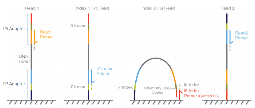
When libraries are prepared using the single-step PCR method, the libraries are constructed slightly different (the colours mentioned refer to the setup described in the two-step approach):

1. Forward Illumina adapter (red)
2. Forward Illumina sequencing primer (orange)
3. Forward barcode sequence (darkgreen)
4. Amplicon (including primers)
5. Reverse barcode sequence (lightgreen)
6. Reverse Illumina sequencing primer (lightblue)
7. Reverse Illumina adapter (darkblue)

In this construction, the barcode sequences are not located in between the Illumina adapter and Illumina sequencing primer, but are said to be ‘inline’. These inline barcode sequences cannot be identified by the Illumina software, since it does not know when the barcode ends and the primer sequence of the amplicon starts. Therefore, this will result in a single sequence file (or two for paired-end sequencing data) containing the data for all samples together. The demultiplexing step, assigning sequences to a sample, will have to be incorporated into the bioinformatic pipeline, something we will cover now in the workshop.

For more information on Illumina sequencing, you can watch the following 5-minute youtube video (EMP). Notice that the ‘Sample Prep’ method described in the video follows the two-step PCR approach.

Assigning sequences to corresponding samples

During library preparation for our sample data, each sample was assigned a specific barcode combination, with at least 3 basepair differences between each barcode used in the library. By searching for these specific sequences, which are situated at the very beginning and very end of each sequence, we can assign each sequence to the corresponding sample. We will be using cutadapt for demultiplexing our dataset today, as it is the fastest option. Cutadapt requires an additional metadata text file in fasta format. This text file contains information about the sample name and the associated barcode and primer sequences.

Let’s have a look at the metadata file, which can be found in the meta subfolder.

$ cd ../meta/
$ ls -ltr

-rw-r--r--@ 1 gjeunen  staff  1139 16 Nov 12:41 sample_metadata.fasta

$ head -10 sample_metadata.fasta

>AM1
GAAGAGGACCCTATGGAGCTTTAGAC;min_overlap=26...AGTTACYHTAGGGATAACAGCGCGACGCTA;min_overlap=30
>AM2
GAAGAGGACCCTATGGAGCTTTAGAC;min_overlap=26...AGTTACYHTAGGGATAACAGCGCGAGTAGA;min_overlap=30
>AM3
GAAGAGGACCCTATGGAGCTTTAGAC;min_overlap=26...AGTTACYHTAGGGATAACAGCGCGAGTCAT;min_overlap=30
>AM4
GAAGAGGACCCTATGGAGCTTTAGAC;min_overlap=26...AGTTACYHTAGGGATAACAGCGCGATAGAT;min_overlap=30
>AM5
GAAGAGGACCCTATGGAGCTTTAGAC;min_overlap=26...AGTTACYHTAGGGATAACAGCGCGATCTGT;min_overlap=30

From the output, we can see that this is a simple two-line fasta format, with the header line containing the sample name info indicated by ”>” and the barcode/primer info on the following line. We can also see that the forward and reverse barcode/primer sequences are split by “…“ and that we specify a minimum overlap between the sequence found in the data file and the metadata file to be the full length of the barcode/primer information.

Count the number of samples in the metadata file

before we get started with our first script, let’s first determine how many samples are included in our experiment.

Hint 1: think about the file structure of the metadata file. Hint 2: a similar line of code can be written to count the number of sequences in a fasta file (which you might have come across before during OBSS2022)

Solution

grep -c "^>" sample_metadata.fasta

grep is a command that searches for strings that match a pattern -c is the parameter indicating to count the number of times we find the pattern "^>" is the string we need to match, in this case >. The ^ indicates that the string needs to occur at the beginning of the line.

Let’s now write our first script to demultiplex our sequence data. First, we’ll navigate to the scripts folder. When listing the files in this folder, we see that a script has already been created, so let’s see what it contains. To read the file, we’ll use the nano function.

$ cd ../scripts/
$ ls -ltr

-rwxrwx--x+ 1 jeuge18p uoo02328 63 Nov 17 13:08 moduleload

$ nano moduleload

#!/bin/bash

module load eDNA/2021.11-gimkl-2020a-Python-3.8.2

Here, we can see that the script starts with what is called a shebang #!, which is to let the computer know how to interpret the script. The following line is specific to NeSI, where we will load the necessary software programs to run our scripts. We will, therefore, add this script to all subsequent scripts to make sure the correct software is available on NeSI.

To exit the script, we can press ctr + X, which will bring us back to the terminal window.

To create a new script to demultiplex our data, we can type the following:

$ nano demux

This command will open the file demux in the nano text editor in the terminal. In here, we can type the following commands:

$ #!/bin/bash
$
$ source moduleload
$
$ cd ../raw/
$
$ cutadapt FTP103_S1_L001_R1_001.fastq.gz -g file:../meta/sample_metadata.fasta -o ../input/{name}.fastq --untrimmed-output untrimmed_FTP103.fastq --no-indels -e 0 --cores=0

We can exit out of the text editor by pressing ctr+X, then type y to save the file, and press enter to save the file as demux. When we list the files in the scripts folder, we can see that this file is now created, but that it is not yet executable (no x in file description).

$ ls -ltr

-rwxrwx--x+ 1 jeuge18p uoo02328  63 Nov 17 13:08 moduleload
-rw-rw----+ 1 jeuge18p uoo02328 210 Nov 17 13:24 demux

To make the script executable, we can use the following code:

$ chmod +x demux

When we now list the files in our scripts folder again, we see that the parameters have changed:

$ ls -ltr

-rwxrwx--x+ 1 jeuge18p uoo02328  63 Nov 17 13:08 moduleload
-rwxrwx--x+ 1 jeuge18p uoo02328 210 Nov 17 13:24 demux

To run the script, we can type:

$ ./demux

Once this script has been executed, it will generate quite a bit of output in the terminal. The most important information, however, can be found at the top, indicating how many sequences could be assigned. The remainder of the output is detailed information for each sample.

This is cutadapt 3.5 with Python 3.8.2
Command line parameters: FTP103_S1_L001_R1_001.fastq.gz -g file:../meta/sample_metadata.fasta -o ../input/{name}.fastq --untrimmed-output untrimmed_FTP103.fastq --no-indels -e 0 --cores=0
Processing reads on 70 cores in single-end mode ...
Done           00:00:07       853,561 reads @   9.3 µs/read;   6.47 M reads/minute
Finished in 7.96 s (9 µs/read; 6.43 M reads/minute).

=== Summary ===

Total reads processed:                 853,561
Reads with adapters:                   128,874 (15.1%)
Reads written (passing filters):       853,561 (100.0%)

Total basepairs processed:   277,407,325 bp
Total written (filtered):    261,599,057 bp (94.3%)

If successfully completed, the script should’ve generated a single fastq file for each sample in the input directory. Let’s list these files and look at the structure of the fastq file:

$ ls -ltr ../input/

-rw-rw----+ 1 jeuge18p uoo02328 5404945 Nov 17 13:31 AM1.fastq
-rw-rw----+ 1 jeuge18p uoo02328 4906020 Nov 17 13:31 AM2.fastq
-rw-rw----+ 1 jeuge18p uoo02328 3944614 Nov 17 13:31 AM3.fastq
-rw-rw----+ 1 jeuge18p uoo02328 5916544 Nov 17 13:31 AM4.fastq
-rw-rw----+ 1 jeuge18p uoo02328 5214931 Nov 17 13:31 AM5.fastq
-rw-rw----+ 1 jeuge18p uoo02328 4067965 Nov 17 13:31 AM6.fastq
-rw-rw----+ 1 jeuge18p uoo02328 4841565 Nov 17 13:31 AS2.fastq
-rw-rw----+ 1 jeuge18p uoo02328 9788430 Nov 17 13:31 AS3.fastq
-rw-rw----+ 1 jeuge18p uoo02328 5290868 Nov 17 13:31 AS4.fastq
-rw-rw----+ 1 jeuge18p uoo02328 5660255 Nov 17 13:31 AS5.fastq
-rw-rw----+ 1 jeuge18p uoo02328 4524100 Nov 17 13:31 AS6.fastq
-rw-rw----+ 1 jeuge18p uoo02328     461 Nov 17 13:31 ASN.fastq

$ head -12 ../input/AM1.fastq

@M02181:93:000000000-D20P3:1:1101:15402:1843 1:N:0:1
GACAGGTAGACCCAACTACAAAGGTCCCCCAATAAGAGGACAAACCAGAGGGACTACTACCCCCATGTCTTTGGTTGGGGCGACCGCGGGGGAAGAAGTAACCCCCACGTGGAACGGGAGCACAACTCCTTGAACTCAGGGCCACAGCTCTAAGAAACAAAATTTTTGACCTTAAGATCCGGCAATGCCGATCAACGGACCG
+
2222E2GFFCFFCEAEF3FFBD32FFEFEEE1FFD55BA1AAEEFFE11AA??FEBGHEGFFGE/F3GFGHH43FHDGCGEC?B@CCCC?C??DDFBF:CFGHGFGFD?E?E?FFDBD.-A.A.BAFFFFFFBBBFFBB/.AADEF?EFFFF///9BBFE..BFFFF;.;FFFB///BBFA-@=AFFFF;-BADBB?-ABD;
@M02181:93:000000000-D20P3:1:1101:16533:1866 1:N:0:1
TTTAGAACAGACCATGTCAGCTACCCCCTTAAACAAGTAGTAATTATTGAACCCCTGTTCCCCTGTCTTTGGTTGGGGCGACCACGGGGAAGAAAAAAACCCCCACGTGGACTGGGAGCACCTTACTCCTACAACTACGAGCCACAGCTCTAATGCGCAGAATTTCTGACCATAAGATCCGGCAAAGCCGATCAACGGACCG
+
GGHCFFBFBB3BA2F5FA55BF5GGEGEEHF55B5ABFB5F55FFBGGB55GEEEFEGFFEFGC1FEFFGBBGH?/??EC/>E/FE???//DFFFFF?CDDFFFCFCF...>DAA...<.<CGHFFGGGH0CB0CFFF?..9@FB.9AFFGFBB09AAB?-/;BFFGB/9F/BFBB/BFFF;BCAF/BAA-@B?/B.-.@DA
@M02181:93:000000000-D20P3:1:1101:18101:1874 1:N:0:1
ACTAGACAACCCACGTCAAACACCCTTACTCTGCTAGGAGAGAACATTGTGGCCCTTGTCTCACCTGTCTTCGGTTGGGGCGACCGCGGAGGACAAAAAGCCTCCATGTGGACTGAAGTAACTATCCTTCACAGCTCAGAGCCGCGGCTCTACGCGACAGAAATTCTGACCAAAAATGATCCGGCACATGCCGATTAACGGAACA
+
BFGBA4F52AEA2A2B2225B2AEEGHFFHHF5BD551331113B3FGDGB??FEGG2FEEGBFFGFGCGHE11FE??//>//<</<///<</CFFB0..<F1FE0G0D000<<AC0<000<DDBC:GGG0C00::C0/00:;-@--9@AFBB.---9--///;F9F//;B/....;//9BBA-9-;.BBBB>-;9A/BAA.999

Renaming sequence headers to incorporate sample names

Before we can continue with the next step in our bioinformatic pipeline, we will need to rename every sequence so that the information of the corresponding sample is incorporated. This will be needed to generate our OTU table at the end of the analysis. Lastly, we can combine all the relabeled files into a single file prior to quality filtering.

$ nano rename

$ #!/bin/bash
$
$ source moduleload
$ 
$ cd ../input/
$
$ for fq in *.fastq; do vsearch --fastq_filter $fq --relabel $fq. --fastqout rl_$fq; done
$
$ cat rl* > ../output/relabel.fastq

$ chmod +x rename

$ ./rename

Once executed, the script will first rename the sequence headers of each file and store them in a new file per sample. Lastly, we have combinned all relabeled files using the cat command. This combined file can be found in the output folder. Let’s see if it is there and how the sequence headers have been altered:

$ ls -ltr ../output/

-rw-rw----+ 1 jeuge18p uoo02328 54738505 Nov 17 13:51 relabel.fastq

head -12 ../output/relabel.fastq

@AM1.fastq.1
GACAGGTAGACCCAACTACAAAGGTCCCCCAATAAGAGGACAAACCAGAGGGACTACTACCCCCATGTCTTTGGTTGGGGCGACCGCGGGGGAAGAAGTAACCCCCACGTGGAACGGGAGCACAACTCCTTGAACTCAGGGCCACAGCTCTAAGAAACAAAATTTTTGACCTTAAGATCCGGCAATGCCGATCAACGGACCG
+
2222E2GFFCFFCEAEF3FFBD32FFEFEEE1FFD55BA1AAEEFFE11AA??FEBGHEGFFGE/F3GFGHH43FHDGCGEC?B@CCCC?C??DDFBF:CFGHGFGFD?E?E?FFDBD.-A.A.BAFFFFFFBBBFFBB/.AADEF?EFFFF///9BBFE..BFFFF;.;FFFB///BBFA-@=AFFFF;-BADBB?-ABD;
@AM1.fastq.2
TTTAGAACAGACCATGTCAGCTACCCCCTTAAACAAGTAGTAATTATTGAACCCCTGTTCCCCTGTCTTTGGTTGGGGCGACCACGGGGAAGAAAAAAACCCCCACGTGGACTGGGAGCACCTTACTCCTACAACTACGAGCCACAGCTCTAATGCGCAGAATTTCTGACCATAAGATCCGGCAAAGCCGATCAACGGACCG
+
GGHCFFBFBB3BA2F5FA55BF5GGEGEEHF55B5ABFB5F55FFBGGB55GEEEFEGFFEFGC1FEFFGBBGH?/??EC/>E/FE???//DFFFFF?CDDFFFCFCF...>DAA...<.<CGHFFGGGH0CB0CFFF?..9@FB.9AFFGFBB09AAB?-/;BFFGB/9F/BFBB/BFFF;BCAF/BAA-@B?/B.-.@DA
@AM1.fastq.3
ACTAGACAACCCACGTCAAACACCCTTACTCTGCTAGGAGAGAACATTGTGGCCCTTGTCTCACCTGTCTTCGGTTGGGGCGACCGCGGAGGACAAAAAGCCTCCATGTGGACTGAAGTAACTATCCTTCACAGCTCAGAGCCGCGGCTCTACGCGACAGAAATTCTGACCAAAAATGATCCGGCACATGCCGATTAACGGAACA
+
BFGBA4F52AEA2A2B2225B2AEEGHFFHHF5BD551331113B3FGDGB??FEGG2FEEGBFFGFGCGHE11FE??//>//<</<///<</CFFB0..<F1FE0G0D000<<AC0<000<DDBC:GGG0C00::C0/00:;-@--9@AFBB.---9--///;F9F//;B/....;//9BBA-9-;.BBBB>-;9A/BAA.999

Key Points

• First key point. Brief Answer to questions. (FIXME)

Quality filtering

Overview

Teaching: 15 min
Exercises: 30 min

Questions

• What parameters to use to filter metabarcoding data on quality?

Objectives

• Learn to filter sequences on quality using the VSEARCH pipeline

Quality filtering

Introduction

During the quality filtering step, we will discard all sequences that do not adhere to a specific set of rules. We will be using the program VSEARCH (EMP) for this step. During quality filtering, we will filter out all sequences that do not adhere to a minimum and maximum length, have unassigned base calls (‘N’), and have a higher expected error than 1. Once we have filtered our data, we can check the quality with FastQC and compare it to the raw sequencing file.

Filtering sequence data

$ nano qual

$ #!/bin/bash
$
$ source moduleload
$
$ cd ../output/
$
$ vsearch --fastq_filter relabel.fastq --fastq_maxee 1.0 --fastq_maxlen 230 --fastq_minlen 150 --fastq_maxns 0 --fastaout filtered.fasta --fastqout filtered.fastq

$ chmod +x qual

$ ./qual

vsearch v2.17.1_linux_x86_64, 503.8GB RAM, 72 cores
https://github.com/torognes/vsearch

Reading input file 100%  
123537 sequences kept (of which 0 truncated), 5337 sequences discarded.

After quality filtering, we have 123,537 sequences left over in the fastq and fasta files. Before we continue with the pipeline, let’s check if the quality filtering was successful using FastQC.

nano qualcheck

#!/bin/bash

source moduleload

cd ../output/

fastqc filtered.fastq -o ../meta/

$ chmod +x qualcheck

$ ./qualcheck

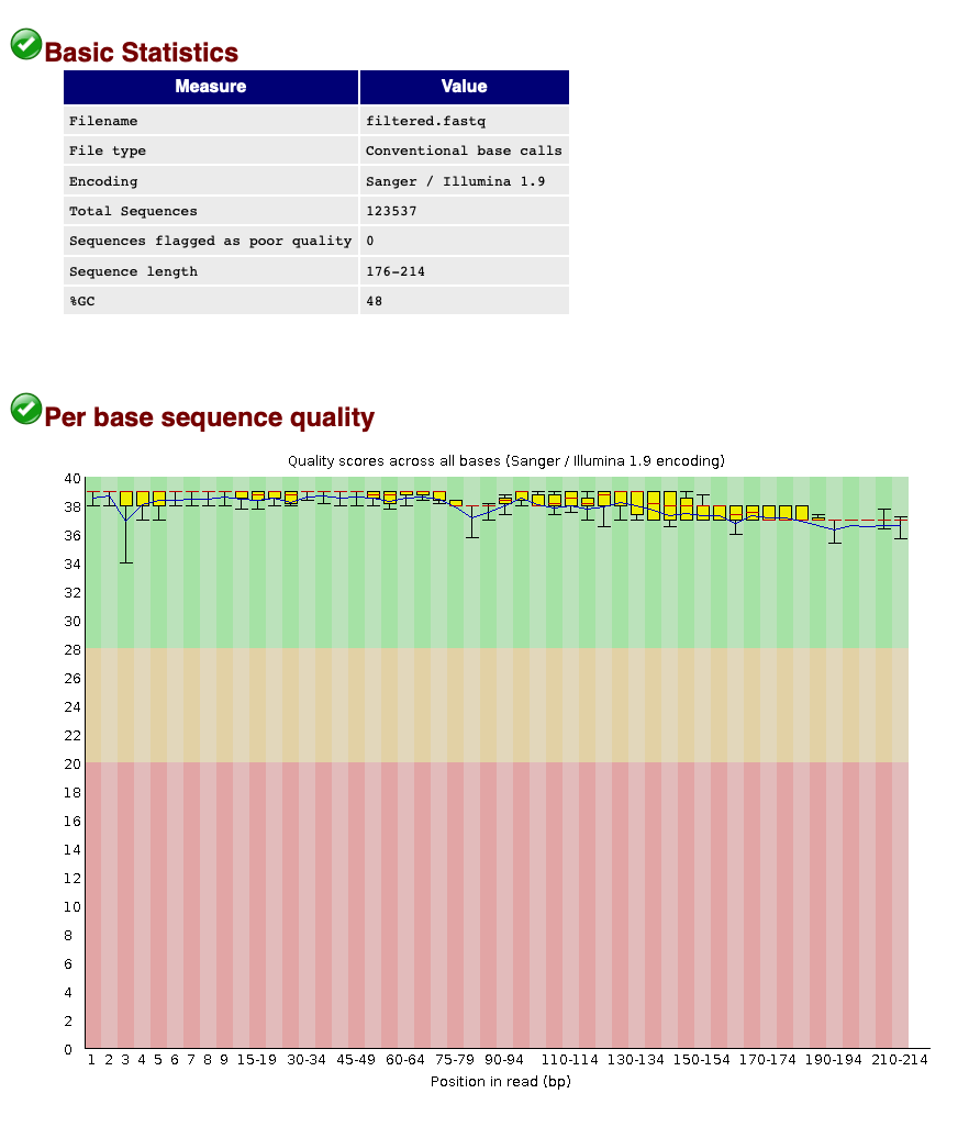
When we now look at the Basic Statistics and Per base sequence quality tabs, we can see that:

1. Our total number of sequences has been reduced to 123,537, similar to the number specified by our qual script.
2. The sequence length ranges from 176-214, according to amplicon length and within the range of the parameters chosen in the qual script.
3. The sequence quality is high throughout the amplicon length (within the green zone).

We can, therefore, conclude that quality filtering was successful and we can now move to the clustering step of the pipeline.

Count the number of sequences in a fastq file

before we continue with our bioinformatic pipeline, let’s first determine how to count the number of sequences in a fastq file in the terminal

Hint 1: think about the file structure of the fastq file. Hint 2: think about how to calculate number of sequences in a fasta file

Solution

grep -c "^@" filtered.fastq

Key Points

• Quality filtering on sequence length, ambiguous basecalls, and maximum error rate

OTU clustering

Overview

Teaching: 15 min
Exercises: 30 min

Questions

• Is it better to denoise or cluster sequence data?

Objectives

• Learn to cluster sequences into OTUs with the VSEARCH pipeline

OTU clustering

Introduction

Now that the dataset is filtered and each sequence is assigned to their corresponding sample, we are ready for the next step in the bioinformatic pipeline, i.e., looking for biologically meaningful or biologically correct sequences. This is done through denoising or clustering the dataset, while at the same time removing any chimeric sequences and remaining PCR and/or sequencing errors.

There is still an ongoing debate on what the best approach is to obtain these biologically meaningful sequences. If you would like more information, these are two good papers to start with paper 1 (EMP); paper 2 (EMP). We won’t be discussing this topic in much detail during the workshop, but this is the basic idea…

When clustering the dataset, OTUs (Operational Taxonomic Units) will be generated by combining sequences that are similar to a set percentage level (traditionally 97%), with the most abundant sequence identified as the true sequence. When clustering at 97%, this means that if a sequence is more than 3% different than the generated OTU, a second OTU will be generated. The concept of OTU clustering was introduced in the 1960s and has been debated since. Clustering the dataset is usually used for identifying species in metabarcoding data.

Denoising, on the other hand, attempts to identify all correct biological sequences through an algorithm, which his visualised in the figure below. In short, denoising will cluster the data with a 100% threshold and tries to identify errors based on abundance differences. The retained sequences are called ZOTU (Zero-radius Operation Taxonomic Unit) or ASVs (Amplicon Sequence Variants). Denoising the dataset is usually used for identifying intraspecific variation in metabarcoding data.

This difference in approach may seem small but has a very big impact on your final dataset!

When you denoise the dataset, it is expected that one species may have more than one ZOTU, while if you cluster the dataset, it is expected that an OTU may have more than one species assigned to it. This means that you may lose some correct biological sequences that are present in your data when you cluster the dataset, because they will be clustered together. In other words, you will miss out on differentiating closely related species and intraspecific variation. For denoising, on the other hand, it means that when the reference database is incomplete, or you plan to work with ZOTUs instead of taxonomic assignments, your diversity estimates will be highly inflated.

For this workshop, we will follow the clustering pathway, since most people are working on vertebrate datasets with good reference databases and are interested in taxonomic assignments.

Dereplicating the data

Before we can cluster our dataset, we need to dereplicate the sequences into unique sequences. Since metabarcoding data is based on an amplification method, the same DNA molecule can be sequenced several times. In order to reduce file size and computational time, it is convenient to work with unique sequences.

During dereplication, we will remove unique sequences that are not prevalent in our dataset. There is still not a standardised guide to the best cutoff. Many eDNA metabarcoding publications remove only the singleton sequences, i.e., sequences that are present once in the dataset, while others opt to remove unique sequences occurring less than three or ten times. Given there isn’t a standard approach, we will be using the more strict approach of removing sequences occurring fewer than 10 times in the dataset. Lastly, we will sort the sequences based on abundance, as this will be needed for the OTU clustering step.

nano derep

#!/bin/bash

source moduleload

cd ../output/

vsearch --derep_fulllength filtered.fasta --relabel uniq. --output uniques.fasta --sizeout --minuniquesize 10

vsearch --sortbysize uniques.fasta --output sorted_uniques.fasta

chmod +x derep
./derep

vsearch v2.17.1_linux_x86_64, 503.8GB RAM, 72 cores
https://github.com/torognes/vsearch

Dereplicating file filtered.fasta 100%  
25083932 nt in 123537 seqs, min 176, max 214, avg 203
Sorting 100%
6645 unique sequences, avg cluster 18.6, median 1, max 19554
Writing output file 100% 
286 uniques written, 6359 clusters discarded (95.7%)
vsearch v2.17.1_linux_x86_64, 503.8GB RAM, 72 cores
https://github.com/torognes/vsearch

Reading file uniques.fasta 100%  
58019 nt in 286 seqs, min 189, max 213, avg 203
Getting sizes 100% 
Sorting 100%
Median abundance: 17
Writing output 100% 

To check if everything executed properly, we can list the files that are in the output folder and check if both output files have been generated (uniques.fasta and sorted_uniques.fasta).

$ ls -ltr ../output/

-rw-rw----+ 1 jeuge18p uoo02328 54738505 Nov 17 13:51 relabel.fastq
-rw-rw----+ 1 jeuge18p uoo02328 27440390 Nov 17 14:31 filtered.fasta
-rw-rw----+ 1 jeuge18p uoo02328 52647859 Nov 17 14:31 filtered.fastq
-rw-rw----+ 1 jeuge18p uoo02328    63983 Nov 17 15:13 uniques.fasta
-rw-rw----+ 1 jeuge18p uoo02328    63983 Nov 17 15:13 sorted_uniques.fasta

We can also check how these commands have altered our files. Let’s have a look at the sorted_uniques.fasta file, by using the head command.

$ head ../output/sorted_uniques.fasta

>uniq.1;size=19554
TTTAGAACAGACCATGTCAGCTACCCCCTTAAACAAGTAGTAATTATTGAACCCCTGTTCCCCTGTCTTTGGTTGGGGCG
ACCACGGGGAAGAAAAAAACCCCCACGTGGACTGGGAGCACCTTACTCCTACAACTACGAGCCACAGCTCTAATGCGCAG
AATTTCTGACCATAAGATCCGGCAAAGCCGATCAACGGACCG
>uniq.2;size=14321
ACTAAGGCATATTGTGTCAAATAACCCTAAAACAAAGGACTGAACTGAACAAACCATGCCCCTCTGTCTTAGGTTGGGGC
GACCCCGAGGAAACAAAAAACCCACGAGTGGAATGGGAGCACTGACCTCCTACAACCAAGAGCTGCAGCTCTAACTAATA
GAATTTCTAACCAATAATGATCCGGCAAAGCCGATTAACGAACCA
>uniq.3;size=8743
ACCAAAACAGCTCCCGTTAAAAAGGCCTAGATAAAGACCTATAACTTTCAATTCCCCTGTTTCAATGTCTTTGGTTGGGG

Study Questions 1

What do you think the following parameters are doing?

• --sizeout
• --minuniquesize 2
• --relabel Uniq.

Solution

--sizeout: this will print the number of times a sequence has occurred in the header information. You can use the head command on the sorted file to check how many times the most abundant sequence was encountered in our sequencing data.

--minuniquesize 2: only keeps the dereplicated sequences if they occur twice or more. To check if this actually happened, you can use the tail command on the sorted file to see if there are any dereplicates sequences with --sizeout 1.

--relabel Uniq.: this parameter will relabel the header information to Uniq. followed by an ascending number, depending on how many different sequences have been encountered.

Chimera removal and clustering

Now that we have dereplicated and sorted our sequences, we can remove chimeric sequences, cluster our data to generate OTUs, and generate a frequency table. We will do this by writing the following script:

nano cluster

#!/bin/bash

source moduleload

cd ../output/

vsearch --uchime3_denovo sorted_uniques.fasta --nonchimeras nonchimeras.fasta

vsearch --cluster_size nonchimeras.fasta --centroids ../final/otus.fasta --relabel otu. --id 0.97

vsearch --usearch_global filtered.fasta --db ../final/otus.fasta --strand plus --otutabout ../final/otutable.txt --id 0.97

chmod +x cluster
./cluster

vsearch v2.17.1_linux_x86_64, 503.8GB RAM, 72 cores
https://github.com/torognes/vsearch

Reading file sorted_uniques.fasta 100%  
58019 nt in 286 seqs, min 189, max 213, avg 203
Masking 100% 
Sorting by abundance 100%
Counting k-mers 100% 
Detecting chimeras 100%  
Found 28 (9.8%) chimeras, 258 (90.2%) non-chimeras,
and 0 (0.0%) borderline sequences in 286 unique sequences.
Taking abundance information into account, this corresponds to
885 (0.8%) chimeras, 111140 (99.2%) non-chimeras,
and 0 (0.0%) borderline sequences in 112025 total sequences.
vsearch v2.17.1_linux_x86_64, 503.8GB RAM, 72 cores
https://github.com/torognes/vsearch

Reading file nonchimeras.fasta 100%  
52356 nt in 258 seqs, min 189, max 213, avg 203
Masking 100% 
Sorting by abundance 100%
Counting k-mers 100% 
Clustering 100%  
Sorting clusters 100%
Writing clusters 100% 
Clusters: 26 Size min 1, max 58, avg 9.9
Singletons: 5, 1.9% of seqs, 19.2% of clusters
vsearch v2.17.1_linux_x86_64, 503.8GB RAM, 72 cores
https://github.com/torognes/vsearch

Reading file ../final/otus.fasta 100%  
5277 nt in 26 seqs, min 189, max 213, avg 203
Masking 100% 
Counting k-mers 100% 
Creating k-mer index 100% 
Searching 100%  
Matching unique query sequences: 122096 of 123537 (98.83%)
Writing OTU table (classic) 100%  

Once successfully executed, we have generated a list of 26 OTUs and an OTU table containing a combined total of 122,096 sequences.

Study Questions 2

The results of the last script creates three files: nonchimeras.fasta, otus.fasta, and otutable.txt. Let’s have a look at these files to see what the output looks like. From looking at the output, can you guess what some of these VSEARCH parameters are doing?

• --sizein
• --sizeout
• --centroids
• --relabel

How about --fasta_width 0? Try rerunning the script without this command to see if you can tell what this option is doing.

Hint: you can always check the help documentation of the module by loading the module source moduleload and calling the help documentation vsearch -h or by looking at the manual of the software, which can usually be found on the website.

Optional extra 1

We discussed the difference between denoising and clustering. You can change the last script to have VSEARCH do denoising instead of clustering. Make a new script to run denoising. It is similar to cluster, except you do not use the vsearch --cluster_size command. Instead you will use:

vsearch --cluster_unoise sorted_uniques.fasta --sizein --sizeout --fasta_width 0 --centroids centroids_unoise.fasta

You will still need the commands to remove chimeras and create a frequency table. Make sure to change the names of the files so that you are making a new frequency table and OTU fasta file (maybe call it asvs.fasta). If you leave the old name in, it will be overwritten when you run this script.

Give it a try and compare the number of OTUs between clustering and denoising outputs.

Optional extra 2

The --id argument is critical for clustering. What happens if you raise or lower this number? Try rerunning the script to see how it changes the results. Note: make sure to rename the output each time or you will not be able to compare to previous runs.

Key Points

• Clustering sequences into OTUs can miss closely related species

• Denoising sequences can create overestimate diversity when reference databases are incomplete

Creating A Reference Database

Overview

Teaching: 15 min
Exercises: 30 min

Questions

• What reference databases are available for metabarcoding

• How do I make a custom database?

Objectives

• First learning objective. (FIXME)

Reference databases

Introduction

As we have previously discussed, eDNA metabarcoding is the process whereby we amplify a specific gene region of the taxonomic group of interest from an environmental sample. Once the DNA is amplified, we sequence it and up till now, we have been filtering the data based on quality and assigned sequences to samples. The next step in the bioinformatic process will be to assign a taxonomy to each of the sequences, so that we can determine what species are detected through our eDNA analysis.

There are multiple ways to assign taxonomy to a sequence. While this workshop won’t go into too much detail about the different taxonomy assignment methods, any method used will require a reference database.

Several reference databases are available online. The most notable ones being NCBI, EMBL, BOLD, SILVA, and RDP. However, recent research has indicated a need to use custom curated reference databases to increase the accuracy of taxonomy assignment. While certain reference databases are available (RDP: 16S microbial; MIDORI: COI eukaryotes; etc.), this necessary data source is missing in most instances. We will, therefore, show you how to build your own custom curated reference database using a program we developed and was recently accepted for publication in Molecular Ecology Resources, called CRABS: Creating Reference databases for Amplicon-Based Sequencing. For this workshop, we’ll be using an older version of CRABS that is installed on NeSI. However, if you’d like to try making your own reference database for your own study, we suggest to install it on your computer via Docker, conda, or GitHub (CRABS (EMP)).

CRABS - a new program to build custom reference databases

The CRABS workflow consists of seven parts, including:

• (i) downloading and importing data from online repositories into CRABS;
• (ii) retrieving amplicon regions through in silico PCR analysis;
• (iii) retrieving amplicons with missing primer-binding regions through pairwise global alignments using results from in silico PCR analysis as seed sequences;
• (iv) generating the taxonomic lineage for sequences;
• (v) curating the database via multiple filtering parameters;
• (vi) post-processing functions and visualizations to provide a summary overview of the final reference database; and
• (vii) saving the database in various formats covering most format requirements of taxonomic assignment tools.

Today, we will build a custom curated reference database of shark (Chondrichthyes) sequences from the 16S gene region. The reason why we’re focusing on sharks in this tutorial, is that the dataset needed to be downloaded from NCBI is small and won’t overload the NCBI servers if we download sequences all together. Since our sample data includes both fish and sharks, we have placed a CRABS-generated reference databases containing fish and sharks already in the refdb folder that we will be using during taxonomy assignment.

Before we get started, we will quickly go over the help information of the program. As before, we will first have to source the moduleload script to load the program.

source moduleload
crabs -h

usage: crabs [-h] [--version] {db_download,db_import,db_merge,insilico_pcr,pga,assign_tax,dereplicate,seq_cleanup,db_subset,visualization,tax_format} ...

creating a curated reference database

positional arguments:
  {db_download,db_import,db_merge,insilico_pcr,pga,assign_tax,dereplicate,seq_cleanup,db_subset,visualization,tax_format}

optional arguments:
  -h, --help            show this help message and exit
  --version             show program's version number and exit

As you can see, the help documentation shows you how to use the program, plus displays all the functions that are currently available within CRABS. To display the help documentation of a function, we can type the following command:

crabs db_download -h

usage: crabs db_download [-h] -s SOURCE [-db DATABASE] [-q QUERY] [-o OUTPUT] [-k ORIG] [-d DISCARD] [-e EMAIL] [-b BATCHSIZE]

downloading sequence data from online databases

optional arguments:
  -h, --help            show this help message and exit
  -s SOURCE, --source SOURCE
                        specify online database used to download sequences. Currently supported options are: (1) ncbi, (2) embl, (3) mitofish, (4) bold, (5) taxonomy
  -db DATABASE, --database DATABASE
                        specific database used to download sequences. Example NCBI: nucleotide. Example EMBL: mam*. Example BOLD: Actinopterygii
  -q QUERY, --query QUERY
                        NCBI query search to limit portion of database to be downloaded. Example: "16S[All Fields] AND ("1"[SLEN] : "50000"[SLEN])"
  -o OUTPUT, --output OUTPUT
                        output file name
  -k ORIG, --keep_original ORIG
                        keep original downloaded file, default = "no"
  -d DISCARD, --discard DISCARD
                        output filename for sequences with incorrect formatting, default = not saved
  -e EMAIL, --email EMAIL
                        email address to connect to NCBI servers
  -b BATCHSIZE, --batchsize BATCHSIZE
                        number of sequences downloaded from NCBI per iteration. Default = 5000

Step 1: download sequencing data from online repositories

As a first step, we will download the 16S shark sequences from NCBI. While there are multiple repositories supported by CRABS, we’ll focus on this one today.

crabs db_download -s ncbi -db nucleotide -q '16S[All Fields] AND ("Chondrichthyes"[Organism] OR Chondrichthyes[All Fields])' -o sharks_16S_ncbi.fasta -e johndoe@gmail.com

Let’s look at the top 2 lines of the downloaded fasta file to see what CRABS created:

head -2 sharks_16S_ncbi.fasta

>LC738810
ATCCCAGTGAGATCGCCCCTACTCATCCTTTAAGAAAACAGGGAGCAGGTATCAGGCACGCCCCTATCAGCCCAAGACACCTTGCTTAGCCACGCCCCCAAGGGACTTCAGCAGTGATTAATATTAGATAATGAACGAAAGTTTGATCTAGTTAAGGTTATTAGAGCCGGCCAACCTCGTGCCAGCCGCCGCGGTTATACGAGCGGCCCAAATTAATGAGATAACGGCGTAAAGAGTGTATAAGAAAAACCTTCCCCTATTAAAGATAAAATAGTGCCCAACTGTTATACGCACCCGCACCAATGAAATCCATTACAAAAGGAACTTTATTATAACAAGGCCTCTTAAAACACGATAGCTAAAAAACAAACTGGGATTAGATACCCCACTATGTTTAGCCCTAAACCTAGGTGTTTAATTACCCAAACACCCGCCAGAGAACTACAAGCGCCAGCTTAAAACCCAAAGGACTTGGCGGTGCCTTAGACCCCCCTAGAGGAGCCTGTTCTAGAACCGATAATCCACGTTCAACCTCACCACCCCTTGCTCTTTCAGCCTATATACCGCCGTCGCCAGCCTGCCCCATGAGGGTCAAACAGCAAGCACAAAGAATTAAACTCCAAAACGTCAGGTCGAGGTGTAGCCCATGAGGTGGGAAGAAATGAGCTACATTTTCTATTAAGATAAACAGATAAATAATGAAATTAAATTTGAAGTTGGATTTAGCAGTAAGATATAAATAGTATATTAATCTGAAAATGGCTCTGAGGCGCGCACACACCGCCCGTCACTCTCCTTAACAAATTAATTAAATATATAATAAAATACTCAAATAAGAGGAGGCAAGTCGTAACATGGTAAGCGTACTGGAAAGTGCGCTTGGAATCAAAATGTAGTTAAAAAGTACAACACCCCCCTTACACAGAGGAAATATCCATGCAAGTCGGATCATTTTGAACTTTATAGTTAACCCAATACACCCGATTAATTATAATCCCCCCCCAAAACGATTTTTAAAAATTAACCAAAACATTTATTATTCTTAGTATAGGAGATAGAAAAG

Here, we can see that the CRABS format is a simple 2-line fasta format with accession numbers as headers and the sequence on the line below.

Step 2: extract amplicon regions through in silico PCR analysis

Once we have downloaded the sequencing data, we can start with a first curation step of the reference database. We will be extracting the amplicon region from each sequence through an in silico PCR analysis. With this analysis, we will locate the forward and reverse primer binding regions and extract the sequence in between. This will significantly reduce file sizes when larger data sets are downloaded, while also keeping only the necessary information.

The information on the primer sequences can be found in the text file crabs_primer_info.txt. Use the head command to visualise the information and copy paste it in the code.

crabs insilico_pcr -h

usage: crabs insilico_pcr [-h] -i INPUT -o OUTPUT -f FWD -r REV [-e ERROR] [-t THREADS]

curating the downloaded reference sequences with an in silico PCR

optional arguments:
  -h, --help            show this help message and exit
  -i INPUT, --input INPUT
                        input filename
  -o OUTPUT, --output OUTPUT
                        output file name
  -f FWD, --fwd FWD     forward primer sequence in 5-3 direction
  -r REV, --rev REV     reverse primer sequence in 5-3 direction
  -e ERROR, --error ERROR
                        number of errors allowed in primer-binding site. Default = 4.5
  -t THREADS, --threads THREADS
                        number of threads used to compute in silico PCR. Default = autodetection

crabs insilico_pcr -i sharks_16S_ncbi.fasta -o sharks_16S_ncbi_insilico.fasta -f GACCCTATGGAGCTTTAGAC -r CGCTGTTATCCCTADRGTAACT

Step 3: assigning a taxonomic lineage to each sequence

Before we continue curating the reference database, we will need assign a taxonomic lineage to each sequence. The reason for this is that we have the option to curate the reference database on the taxonomic ID of each sequence. For this module, we normally need to download the taxonomy files from NCBI using the db_download --source taxonomy function. However, these files are already available to you for this tutorial. Therefore, we can skip the download of these files. CRABS extracts the necessary taxonomy information from these NCBI files to provide a taxonomic lineage for each sequence using the assign_tax function.

Let’s call the help documentation of the assign_tax function to see what parameters we need to fill in.

crabs assign_tax -h

usage: crabs assign_tax [-h] -i INPUT -o OUTPUT -a ACC2TAX -t TAXID -n NAME [-w WEB] [-r RANKS] [-m MISSING]

creating the reference database with taxonomic information

optional arguments:
  -h, --help            show this help message and exit
  -i INPUT, --input INPUT
                        input file containing the curated fasta sequences after in silico PCR
  -o OUTPUT, --output OUTPUT
                        curated reference database output file
  -a ACC2TAX, --acc2tax ACC2TAX
                        accession to taxid file name
  -t TAXID, --taxid TAXID
                        taxid file name
  -n NAME, --name NAME  phylogeny file name
  -w WEB, --web WEB     retrieve missing taxonomic information through a web search. Default = "no"
  -r RANKS, --ranks RANKS
                        taxonomic ranks included in the taxonomic lineage. Default = "superkingdom+phylum+class+order+family+genus+species"
  -m MISSING, --missing MISSING
                        filename for sequences for which CRABS could not generate a taxonomic lineage (e.g., novel species, typo in species name)

crabs assign_tax -i sharks_16S_ncbi_insilico.fasta -o sharks_16S_ncbi_insilico_tax.tsv -a nucl_gb.accession2taxid -t nodes.dmp -n names.dmp

The output file of the assign_tax function is a tab-delimited file, whereby taxonomy information and sequence is all encountered on a single line. Let’s use the head function to determine the structure:

head -10 sharks_16S_ncbi_insilico_tax.tsv

OM687170	1206156	Eukaryota	Chordata	Chondrichthyes	Myliobatiformes	Myliobatidae	Rhinoptera	Rhinoptera_brasiliensis	ACTTAAGTTACCTTTAAAATATTAAATTTAACCCCCTTTGGGCATAAATAATAAACTAATTTCCTAACTTAACTTGTTTTTGGTTGGGGCGACCAAGGGGAAAAACAAAACCCCCTTACCGAATGTGTGAGATATCACTTAAAAATTAGAGTCACATCTCTAATCAATAGAAAATCTAACGAACAATGACCCAGGAATCCATTTATCCTGATCAATGAACCA
OP391486	195309	Eukaryota	Chordata	Chondrichthyes	Chimaeriformes	Chimaeridae	Hydrolagus	Hydrolagus_mitsukurii	AATATATTAATAAAAGGAATTTAGAACCCTCAGGGGATAAGAAATGGACTTAGCATAATAAAATTATTTTTGGTTGGGGCAACCACGGGGTATAACCTAACCCCCGTATCGATTGGGCAAAAAATGCCTAAAAAATAGAACGACAGTTCTATTTAATAAAATATTTAACGAGTAACGATCCAGAGATATCTGATTAATGAACCA
NC_066805	68454	Eukaryota	Chordata	Chondrichthyes	Carcharhiniformes	Scyliorhinidae	Scyliorhinus	Scyliorhinus_stellaris	ACATAAATTAATTATGTACATATTAATAATCCCAGGACATAAACAAAAAATATAATATTTCTAATTTAACTATTTTTGGTTGGGGTGACCAAGGGGAAAAATGAATCCCCCTTATCGACCGAGTATTCAAGTACTTAAAAGTTAGAATTACAATTCTAACCGATAAAATTTTTACCGAAAAATGACCCAGGATTTTCCTGATCAATGAACCA
NC_066688	195333	Eukaryota	Chordata	Chondrichthyes	Rhinopristiformes	Rhynchobatidae	Rhynchobatus	Rhynchobatus_djiddensis	ACTTAAGTTAATTACTCCATATAAACCACCCCTCCGGGTATAAAACAACATAAATAAATCTAACTTAACTTGTTTTTGGTTGGGGCGACCAAGGGGAAAAACAAAACCCCCTTATCGATTGAGTATTCAACATACTTAAAAATTAAAACGAATAGTTTTAATTAATAGAACATCTAACGAACAATGACCCAGGACACATCCTGATCAATGAACCA
MN389524	2060314	Eukaryota	Chordata	Chondrichthyes	Myliobatiformes	Dasyatidae	Neotrygon	Neotrygon_indica	ACTTAAGTTACCTTAACACCAAAAATTACACCCCAGGGTATAAAAACTAGAAATAACCTCTAACTTAACTTGTTTTCGGTTGGGGCGACCAAGGAGTAAAACAAAACCCCCTTATCGAATGTGTGAGAAATCACTCAAAATTAGAATTACAATTCTAATTAATAGAAGATCTAACGAACAATGACCCAGGACCTCATCCTGATCAATGAACCA
OM404361	195316	Eukaryota	Chordata	Chondrichthyes	Torpediniformes	Narcinidae	Narcine	Narcine_timlei	AATTAAATTAATAAAACAAGACATTTTAAACGACAGTTATAAACACACACCTTATTTTAATTTAACATTTTTGGTTGGGGCAACCAAGGGGAACAAAAAAACCCCCTTATCGATTAAGTATTATATGTACTTAAAATAATAGAAAGACTTTTCAAATTTACAGAACATCTGACGAAATATGACCCAAGAATCTTCTTGATCAATGAACCA
LC636781	2704970	Eukaryota	Chordata	Chondrichthyes	Myliobatiformes	Dasyatidae	Hemitrygon	Hemitrygon_akajei	ACTTAAGTTATTTTTAAACATCAAAAATTTCCCACCTTCGGGCATAAAATAACATAAAATAAATCTTCTAACTTAACTTGTTTTTGGTTGGGGCGACCGAGGGGTAAAACAAAACCCCCTTATCGAATGGGTGAGAAATCACTCAAAATTAGAACGACAGTTCTAATTAATAGAAAATCTAACGAACAATGACCCAGGAAACTATATCCTGATCAATGAACCA
ON065568	195333	Eukaryota	Chordata	Chondrichthyes	Rhinopristiformes	Rhynchobatidae	Rhynchobatus	Rhynchobatus_djiddensis	ACTTAAGTTAATTACTCCATATAAACCACCCCTCCGGGTATAAAACAACATAAATAAATCTAACTTAACTTGTTTTTGGTTGGGGCGACCAAGGGGAAAAACAAAACCCCCTTATCGATTGAGTATTCAACATACTTAAAAATTAAAACGAATAGTTTTAATTAATAGAACATCTAACGAACAATGACCCAGGACACATCCTGATCAATGAACCA
ON065567	335006	Eukaryota	Chordata	Chondrichthyes	Rhinopristiformes	Rhynchobatidae	Rhynchobatus	Rhynchobatus_australiae	ACTTAAGTTAATTACTCCATATAAACCACCCCTTCGGGCATAAAACAACATAAATAAATCTAACTTAACTTGTTTTTGGTTGGGGCGACCAAGGGGAAAAACAAAACCCCCTTATCGACTGAGTATTCAACATACTTAAAAATTAAAACGAATAGTTTTAATTAATAGAACATCTAACGAACAATGACCCAGGACACACATCCTGATCAATGAACCA
LC723525	68454	Eukaryota	Chordata	Chondrichthyes	Carcharhiniformes	Scyliorhinidae	Scyliorhinus	Scyliorhinus_stellaris	ACATAAATTAATTATGTACATATTAATAATCCCAGGACATAAACAAAAAATATAATATTTCTAATTTAACTATTTTTGGTTGGGGTGACCAAGGGGAAAAATGAATCCCCCTTATCGACCGAGTATTCAAGTACTTAAAAGTTAGAATTACAATTCTAACCGATAAAATTTTTACCGAAAAATGACCCAGGATTTTCCTGATCAATGAACCA

Count the number of sequences in the output file of the assign_tax function

Before we continue, let’s first determine how many sequences are included in our reference database.

Hint 1: think about the file structure.

Solution

wc -l sharks_16S_ncbi_insilico_tax.tsv

wc is a command that stands for word count -l indicates we want to count lines, rather than words in our document

Step 4: curate the reference database

Next, we will run two different functions to curate the reference database, the first is to dereplicate the data using the dereplicate function, the second is to filter out sequences that we would not want to include in our final database using the seq_cleanup function.

crabs dereplicate -i sharks_16S_ncbi_insilico_tax.tsv -o sharks_16S_ncbi_insilico_tax_derep.tsv -m uniq_species
crabs seq_cleanup -i sharks_16S_ncbi_insilico_tax_derep.tsv -o sharks_16S_ncbi_insilico_tax_derep_clean.tsv -e yes -s yes -na 0

After curation, we’re left with 552 16S shark sequences in our reference database.

Step 5: export the reference database to a format supported by the taxonomy assignment software

Lastly, we can export the reference database to one of several formats that are implemented in the most commonly used taxonomic assignment tools using the tax_format function. Since we’ll be using SINTAX to assign taxonomy to our OTUs in the following section, let’s export our shark database to SINTAX format as well.

crabs tax_format -i sharks_16S_ncbi_insilico_tax_derep_clean.tsv -o sharks_16S_ncbi_insilico_tax_derep_clean_sintax.fasta -f sintax

Let’s open the reference database to see what the final database looks like!

head sharks_16S_ncbi_insilico_tax_derep_clean_sintax.fasta

>OM687170;tax=d:Eukaryota,p:Chordata,c:Chondrichthyes,o:Myliobatiformes,f:Myliobatidae,g:Rhinoptera,s:Rhinoptera_brasiliensis
ACTTAAGTTACCTTTAAAATATTAAATTTAACCCCCTTTGGGCATAAATAATAAACTAATTTCCTAACTTAACTTGTTTTTGGTTGGGGCGACCAAGGGGAAAAACAAAACCCCCTTACCGAATGTGTGAGATATCACTTAAAAATTAGAGTCACATCTCTAATCAATAGAAAATCTAACGAACAATGACCCAGGAATCCATTTATCCTGATCAATGAACCA
>OP391486;tax=d:Eukaryota,p:Chordata,c:Chondrichthyes,o:Chimaeriformes,f:Chimaeridae,g:Hydrolagus,s:Hydrolagus_mitsukurii
AATATATTAATAAAAGGAATTTAGAACCCTCAGGGGATAAGAAATGGACTTAGCATAATAAAATTATTTTTGGTTGGGGCAACCACGGGGTATAACCTAACCCCCGTATCGATTGGGCAAAAAATGCCTAAAAAATAGAACGACAGTTCTATTTAATAAAATATTTAACGAGTAACGATCCAGAGATATCTGATTAATGAACCA
>NC_066805;tax=d:Eukaryota,p:Chordata,c:Chondrichthyes,o:Carcharhiniformes,f:Scyliorhinidae,g:Scyliorhinus,s:Scyliorhinus_stellaris
ACATAAATTAATTATGTACATATTAATAATCCCAGGACATAAACAAAAAATATAATATTTCTAATTTAACTATTTTTGGTTGGGGTGACCAAGGGGAAAAATGAATCCCCCTTATCGACCGAGTATTCAAGTACTTAAAAGTTAGAATTACAATTCTAACCGATAAAATTTTTACCGAAAAATGACCCAGGATTTTCCTGATCAATGAACCA
>NC_066688;tax=d:Eukaryota,p:Chordata,c:Chondrichthyes,o:Rhinopristiformes,f:Rhynchobatidae,g:Rhynchobatus,s:Rhynchobatus_djiddensis
ACTTAAGTTAATTACTCCATATAAACCACCCCTCCGGGTATAAAACAACATAAATAAATCTAACTTAACTTGTTTTTGGTTGGGGCGACCAAGGGGAAAAACAAAACCCCCTTATCGATTGAGTATTCAACATACTTAAAAATTAAAACGAATAGTTTTAATTAATAGAACATCTAACGAACAATGACCCAGGACACATCCTGATCAATGAACCA
>MN389524;tax=d:Eukaryota,p:Chordata,c:Chondrichthyes,o:Myliobatiformes,f:Dasyatidae,g:Neotrygon,s:Neotrygon_indica
ACTTAAGTTACCTTAACACCAAAAATTACACCCCAGGGTATAAAAACTAGAAATAACCTCTAACTTAACTTGTTTTCGGTTGGGGCGACCAAGGAGTAAAACAAAACCCCCTTATCGAATGTGTGAGAAATCACTCAAAATTAGAATTACAATTCTAATTAATAGAAGATCTAACGAACAATGACCCAGGACCTCATCCTGATCAATGAACCA

Let’s also have a look at the fish database

head fish_16S_sintax.fasta

>KY228977;tax=d:Eukaryota,p:Chordata,c:Actinopteri,o:Cypriniformes,f:Gobionidae,g:Microphysogobio,s:Microphysogobio_amurensis
ACAAAATTTAACCACGTTAAACAACTCGACAAAAAGCAAGAACTTAGTGGAGTATAAAATTTTACCTTCGGTTGGGGCGACCACGGAGGAAAAACAAGCCTCCGAGTGGAATGGGGTAAATCCCTAAAACCAAGAGAAACATCTCTAAGCCGCAGAACATCTGACCAATAATGATCCGGCCTCATAGCCGATCAACGAACCA
>KY228987;tax=d:Eukaryota,p:Chordata,c:Actinopteri,o:Scombriformes,f:Scombridae,g:Scomberomorus,s:Scomberomorus_niphonius
ACGAAGGTATGTCATGTTAAGCACCCTAAATAAAGGACTAAACCGATTGAACTATACCCCTATGTCTTTGGTTGGGGCGACCCCGGGGTAACAAAAAACCCCCGAGCGGACTGGAAGTACTAACTTCTAAAACCAAGAGCTGCAGCTCGAACAAACAGAATTTCTGACCAATAAGATCCGGCAACGCCGATCAACGGACCG
>KY230517;tax=d:Eukaryota,p:Chordata,c:Actinopteri,o:Siluriformes,f:Sisoridae,g:Glyptothorax,s:Glyptothorax_cavia
ATAAAGATCACCTATGTCAATGAGCCCCATACGGCAGCAAACTAAATAGCAACTGATCTTAATCTTCGGTTGGGGCGACCACGGGAGAAAACAAAGCTCCCACGCGGACTGGGGTAAACCCTAAAACCAAGAAAAACATTTCTAAGCAACAGAACTTCTGACCATTAAGATCCGGCTACACGCCGACCAACGGACCA
>KY231189;tax=d:Eukaryota,p:Chordata,c:Actinopteri,o:Acipenseriformes,f:Acipenseridae,g:Acipenser,s:Acipenser_gueldenstaedtii_x_Acipenser_baerii
ACAAGATCAACTATGCTATCAAGCCAACCACCCACGGAAATAACAGCTAAAAGCATAATAGTACCCTGATCCTAATGTTTTCGGTTGGGGCGACCACGGAGGACAAAATAGCCTCCATGTCGACGGGGGCACTGCCCCTAAAACCTAGGGCGACAGCCCAAAGCAACAGAACATCTGACGAACAATGACCCAGGCTACAAGCCTGATCAACGAACCA
>KY231824;tax=d:Eukaryota,p:Chordata,c:Actinopteri,o:Cypriniformes,f:Leuciscidae,g:Alburnus,s:Alburnus_alburnus
ACAAAATTCAACCACGTTAAACGACTCTGTAGAAAGCAAGAACTTAGTGGCGGATGAAATTTTACCTTCGGTTGGGGCGACCACGGAGGAGAAAGAAGCCTCCGAGTGGACTGGGCTAAACCCCAAAGCTAAGAGAGACATCTCTAAGCCGCAGAACATCTGACCAAGAATGATCCGACTGAAAGGCCGATCAACGAACCA

That’s all it takes to generate your own reference database. We are now ready to assign a taxonomy to our OTUs that were generated in the previous section!

Key Points

• First key point. Brief Answer to questions. (FIXME)

Taxonomy Assignment

Overview

Teaching: 15 min
Exercises: 30 min

Questions

• What are the main strategies for assigning taxonomy to OTUs?

• What is the difference between Sintax and Naive Bayes?

Objectives

• Assign taxonomy using Sintax

• Use less to explore a long help output

• Write a script to assign taxonomy

Taxonomy Assignment: Different Approaches

There are four basic strategies to taxonomy classification (and endless variations of each of these): sequence similarity (SS), sequence composition (SC), phylogenetic (Ph), and probabilistic (Pr) (Hleap et al., 2021).

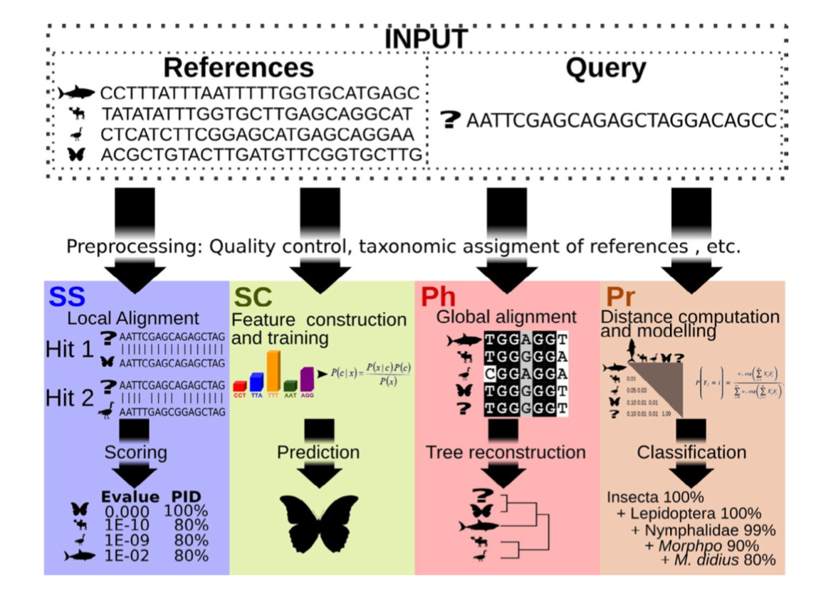
Of the four, the first two are those most often used for taxonomy assignment. For further comparison of these refer to this paper.

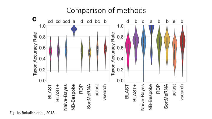
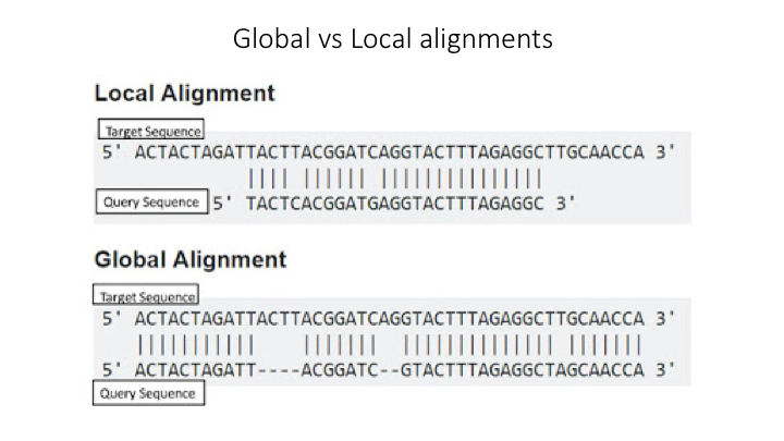
Aligment-Based Methods (SS)

All sequence similarity methods use global or local alignments to directly search a reference database for partial or complete matches to query sequences. BLAST is one of the most common methods of searching DNA sequences. BLAST is an acronym for Basic Local Alignment Search Tool. It is called this because it looks for any short, matching sequence, or local alignments, with the reference. This is contrasted with a global alignment, which tries to find the best match across the entirety of the sequence.

Using Machine Learning to Assign Taxonomy

Sequence composition methods utilise machine learning algorithms to extract compositional features (e.g., nucleotide frequency patterns) before building a model that links these profiles to specific taxonomic groups.

Use the program Sintax to classify our OTUs

The program Sintax is similar to the Naive Bayes classifier used in Qiime and other programs, in that small 8 bp kmers are used to detect patterns in the reference database, but instead of frequency patterns, k-mer similarity is used to identify the top taxonomy, so there is no need for training (Here is a description of the Sintax algorithm). Because of this, it is simplified and can run much faster. Nevertheless, we have found it as accurate as Naive Bayes for the fish dataset we are using in this workshop.

As with the previous steps, we will be using a script to run the classification.

nano taxo

#!/bin/bash

source moduleload

cd ../final/

vsearch --sintax otus.fasta --db ../refdb/fish_16S_sintax.fasta --sintax_cutoff 0.8 --tabbedout taxonomy_otus.txt

chmod +x taxo
./taxo

vsearch v2.17.1_linux_x86_64, 503.8GB RAM, 72 cores
https://github.com/torognes/vsearch

Reading file ../refdb/fish_16S_sintax.fasta 100%  
WARNING: 1 invalid characters stripped from FASTA file: ?(1)
REMINDER: vsearch does not support amino acid sequences
12995009 nt in 75207 seqs, min 101, max 486, avg 173
Counting k-mers 100% 
Creating k-mer index 100% 
Classifying sequences 100%  
Classified 22 of 26 sequences (84.62%)

Taxonomy assignment through SINTAX was able to classify 22 out of 26 OTUs. Now that we have the taxonomy assignment file taxonomy_otus.txt and a frequency table otutable.txt, we have all files needed for the statistical analysis.

Study Questions

Name an OTU that would have better resolution if the cutoff were set to default

Name an OTU that would have worse resolution if the cutoff were set higher

Key Points

• The main taxonomy assignment strategies are global alignments, local alignments, and machine learning approaches

• The main difference is that Naive Bayes requires the reference data to be trained, whereas Sintax looks for only kmer-based matches

Statistics and Graphing with R

Overview

Teaching: 10 min
Exercises: 50 min

Questions

• How do I use ggplot and other programs to visualize metabarcoding data?

• What statistical approaches do I use to explore my metabarcoding results?

Objectives

• Create bar plots of taxonomy and use them to show differences across the metadata

• Create distance ordinations and use them to make PCoA plots

• Compute species richness differences between sampling locations

Statistical analysis in R

In this last section, we’ll go over a bried introduction on how to analyse the data files you’ve created during the bioinformatic analysis, i.e., the frequency table and the taxonomy assignments. Today, we’ll be using R for the statistical analysis, though other options, such as Python, could be used as well. Both of these two coding languages have their benefits and drawbacks, but because most people know R from their Undergraduate classes, we will stick with this option for now.

Please keep in mind that we will only be giving a brief introduction to the statistical analysis. This is by no means a full workshop into how to analyse metabarcoding data. Furthermore, we’ll be sticking to basic R packages to keep things simple and will not go into dedicated metabarcoding packages, such as Phyloseq.

Importing data in R

Before we can analyse our data, we need to import and format the files we created during the bioinformatic analysis, as well as the metadata file. We will also need to load in the necessary R libraries.

###################
## LOAD PACKAGES ##
###################
library('vegan')
library('lattice')
library('ggplot2')
library('labdsv', lib.loc = "/nesi/project/nesi02659/obss_2022/R_lib") # if not on nesi remove lib.loc="..."
library('tidyr')
library('tibble')
library('reshape2')
library('viridis')

#################
## FORMAT DATA ##
#################
## read in the data and metadata
df <- read.delim('../final/otutable.txt', check.names = FALSE, row.names = 1)
tax <- read.delim('../final/taxonomy_otus.txt', check.names = FALSE, row.names = 1, header = FALSE)
meta <- read.csv('metadata.csv', check.names = FALSE)

## merge taxonomy information with OTU table, drop rows without taxID, and sum identical taxIDs
merged <- merge(df, tax, by = 'row.names', all = TRUE)
merged <- subset(merged, select=-c(Row.names,V2, V3))
merged[merged == ''] = NA
merged <- merged %>% drop_na()
merged <- aggregate(. ~ V4, data = merged, FUN = sum)

## remove singleton detections, followed by columns that sum to zero and set taxID as row names
merged[merged == 1] <- 0
merged <- merged[, colSums(merged != 0) > 0]
rownames(merged) <- merged$V4
merged$V4 <- NULL

## transform dataset to presence-absence
merged_pa <- (merged > 0) * 1L 

Preliminary data exploration

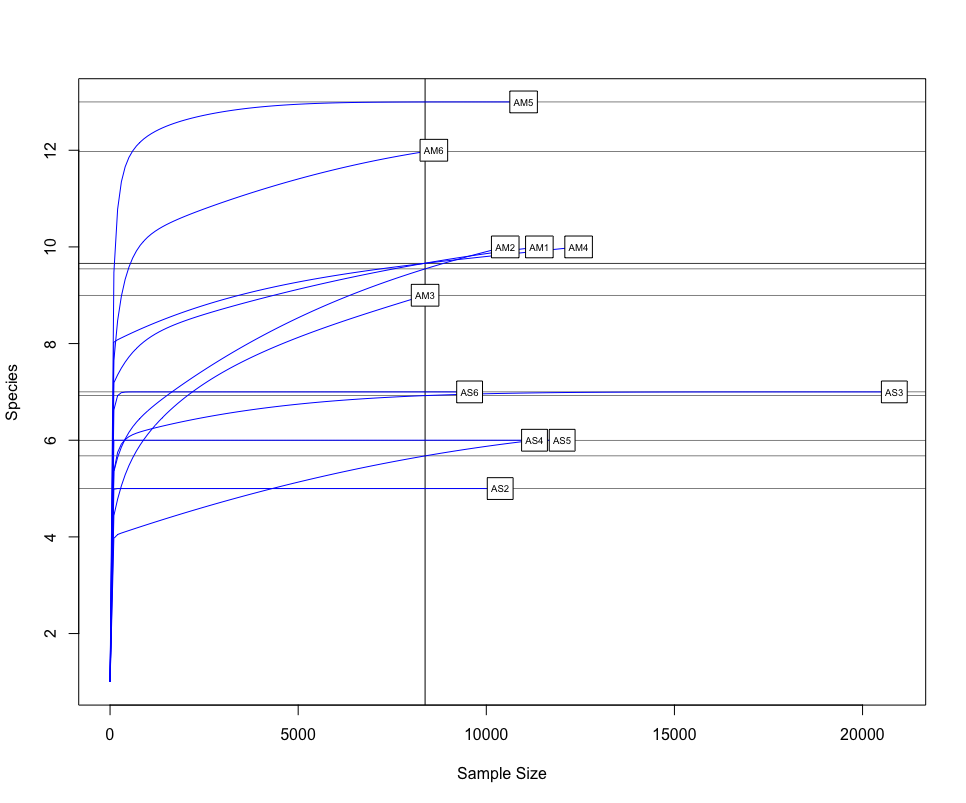
One of the first things we would want to look at, is to determine if sufficient sequencing depth was achieved. We can do this by creating rarefaction curves, which work similar to tradtional species accumulation curves, whereby we randomly select sequences from a sample and determine if new species or OTUs are being detected. If the curve flattens out, it gives the indication sufficient sequencing has been conducted to recover most of the diversity in the dataset.

########################
## RAREFACTION CURVES ##
########################
## transpose the original dataframe and remove negative control
df_t <- t(df)
neg_remove <- c('ASN')
df_t <- df_t[!(row.names(df_t) %in% neg_remove),]

## identify the lowers number of reads for samples and generate rarefaction curves
raremax_df <- min(rowSums(df_t))
rarecurve(df_t, step = 100, sample = raremax_df, col = 'blue', cex = 0.6)

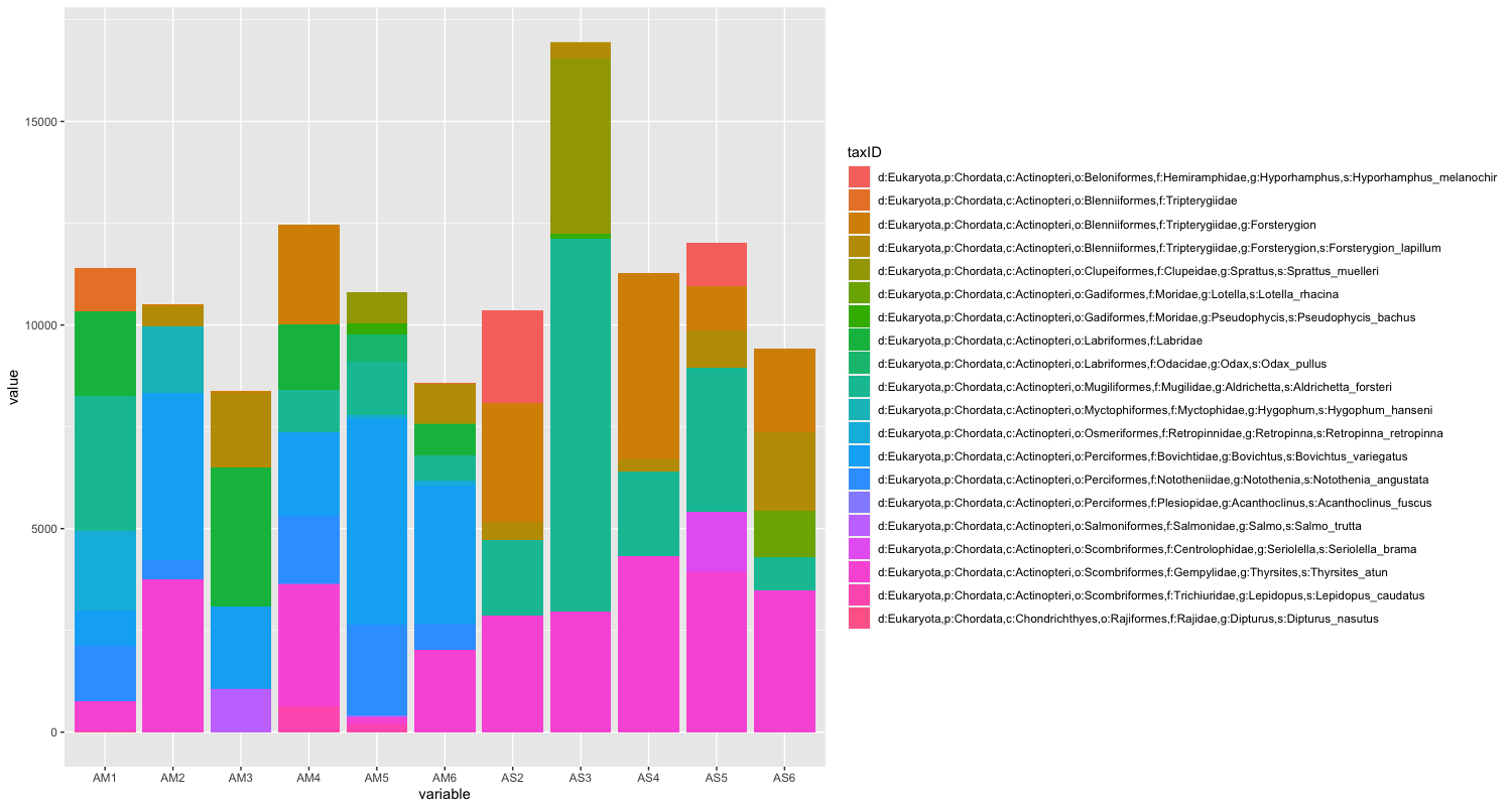
The next step of preliminary data exploration, is to determine what is contained in our data. We can do this by plotting the abundance of each taxon for every sample in a stacked bar plot.

######################
## DATA EXPLORATION ##
######################
## plot abundance of taxa in stacked bar graph
ab_info <- tibble::rownames_to_column(merged, "taxID")
ab_melt <- melt(ab_info)
ggplot(ab_melt, aes(fill = taxID, y = value, x = variable)) +
  geom_bar(position = 'stack', stat = 'identity')

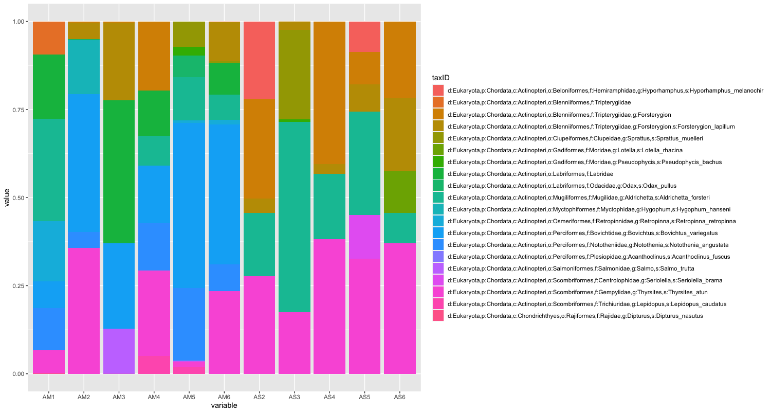
Since the number of sequences differ between samples, it might sometimes be easier to use relative abundances to visualise the data.

## plot relative abundance of taxa in stacked bar graph
ggplot(ab_melt, aes(fill = taxID, y = value, x = variable)) + 
  geom_bar(position="fill", stat="identity")

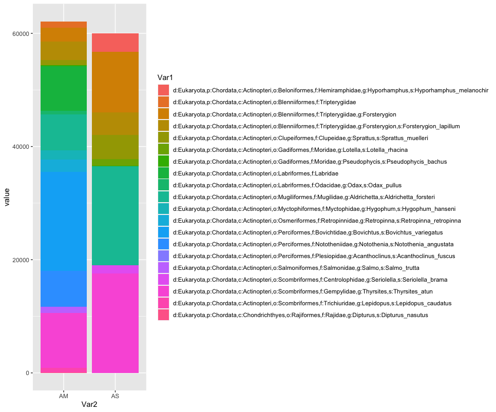
While we can start to see that there are some differences between sampling locations with regards to the observed fish, let’s combine all samples within a sampling location to simplify the graph even further. We can do this by summing or averaging the reads.

# combine samples per sample location and plot abundance and relative abundance of taxa in stacked bar graph
location <- merged
names(location) <- substring(names(location), 1, 2)
locsum <- t(rowsum(t(location), group = colnames(location), na.rm = TRUE))
locsummelt <- melt(locsum)
ggplot(locsummelt, aes(fill = Var1, y = value, x = Var2)) +
  geom_bar(position = 'stack', stat = 'identity')
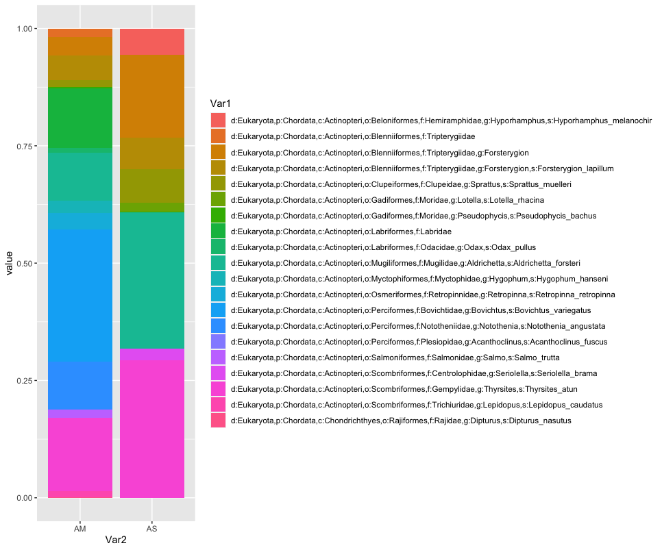
ggplot(locsummelt, aes(fill = Var1, y = value, x = Var2)) + 
  geom_bar(position="fill", stat="identity")

locav <- sapply(split.default(location, names(location)), rowMeans, na.rm = TRUE)
locavmelt <- melt(locav)
ggplot(locavmelt, aes(fill = Var1, y = value, x = Var2)) +
  geom_bar(position = 'stack', stat = 'identity')
ggplot(locavmelt, aes(fill = Var1, y = value, x = Var2)) + 
  geom_bar(position="fill", stat="identity")

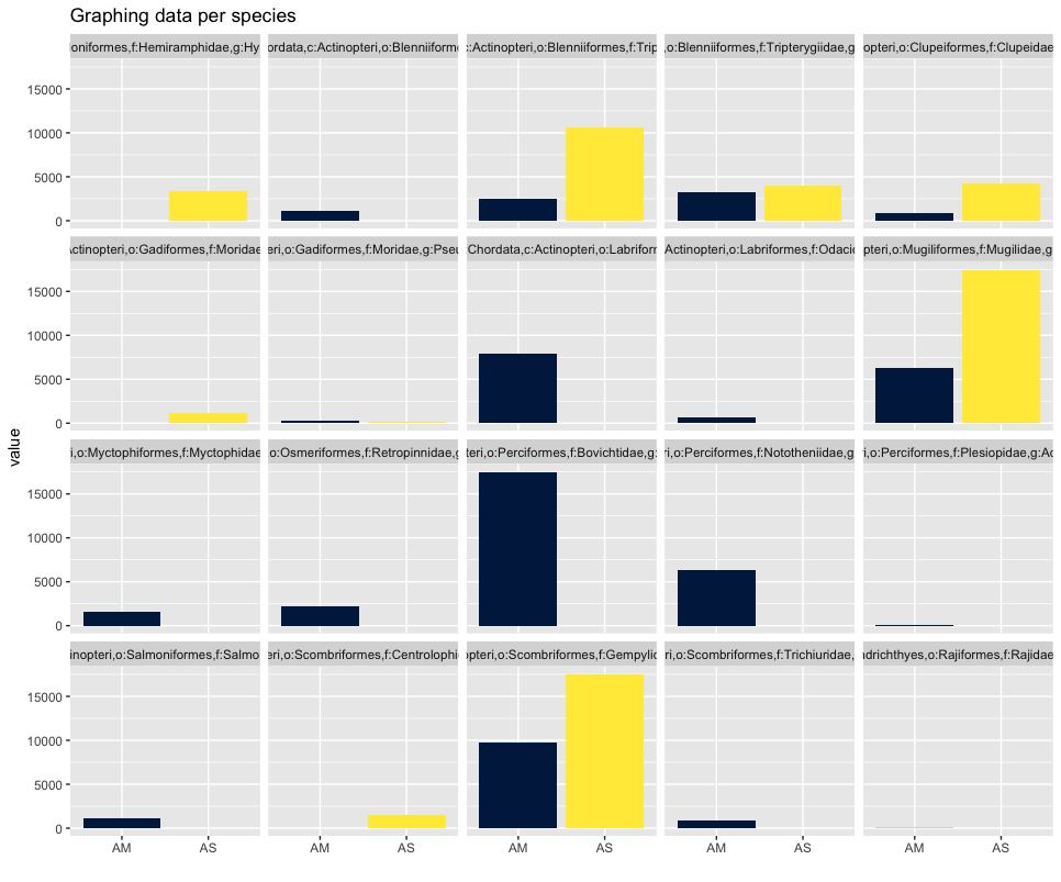
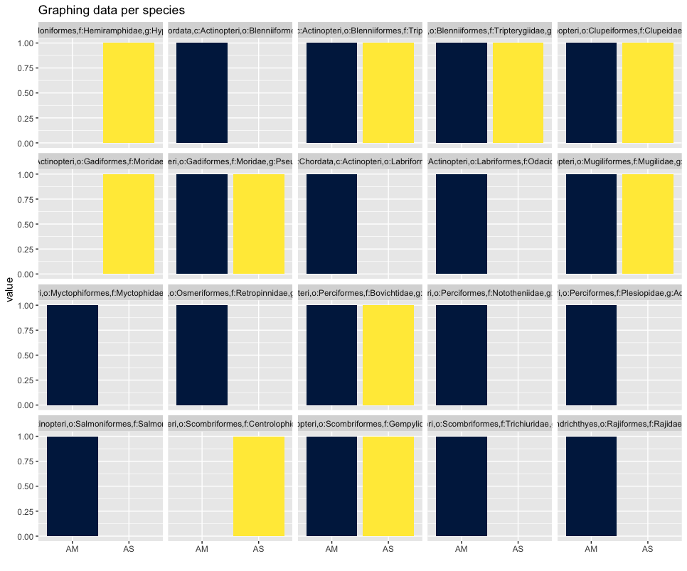
As you can see, the graphs that are produced are easier to interpret, due to the limited number of stacked bars. However, it might still be difficult to identify which species are occurring in only one sampling location, due to the number of species detected and the number of colors used. A trick to use here, is to plot the data per species for the two locations.

## plot per species for easy visualization
ggplot(locsummelt, aes(fill = Var2, y = value, x = Var2)) +
  geom_bar(position = 'dodge', stat = 'identity') +
  scale_fill_viridis(discrete = T, option = "E") +
  ggtitle("Graphing data per species") +
  facet_wrap(~Var1) +
  theme(legend.position = "non") +
  xlab("")

Plotting the relative abundance (transforming it indirectly to presence-absence) could help with distinguishing presence or absence in a sampling location, which could be made difficult due to the potentially big difference in read number.

## plotting per species on relative abundance allows for a quick assessment 
## of species occurrence between locations
ggplot(locsummelt, aes(fill = Var2, y = value, x = Var2)) +
  geom_bar(position = 'fill', stat = 'identity') +
  scale_fill_viridis(discrete = T, option = "E") +
  ggtitle("Graphing data per species") +
  facet_wrap(~Var1) +
  theme(legend.position = "non") +
  xlab("")

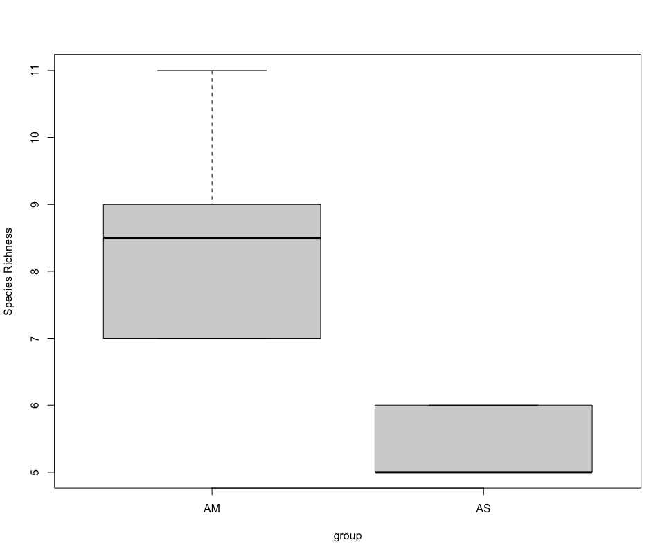
Alpha diversity analysis

Since the correlation between species abudance/biomass and eDNA signal strength has not yet been proven, alpha diversity analysis for metabarcoding data is currently restricted to species richness comparison. In the near future, however, we hope the abundance correlation is proven, enabling more extensive alpha diversity analyses.

######################
## SPECIES RICHNESS ##
######################
## calculate number of taxa detected per sample and group per sampling location
specrich <- setNames(nm = c('colname', 'SpeciesRichness'), stack(colSums(merged_pa))[2:1])
specrich <- transform(specrich, group = substr(colname, 1, 2))

## test assumptions of statistical test, first normal distribution, next homoscedasticity
histogram(~ SpeciesRichness | group, data = specrich, layout = c(1,2))
bartlett.test(SpeciesRichness ~ group, data = specrich)

## due to low sample number per location and non-normal distribution, run Welch's t-test and visualize using boxplot
stat.test <- t.test(SpeciesRichness ~ group, data = specrich, var.equal = FALSE, conf.level = 0.95)
stat.test
boxplot(SpeciesRichness ~ group, data = specrich, names = c('AM', 'AS'), ylab = 'Species Richness')

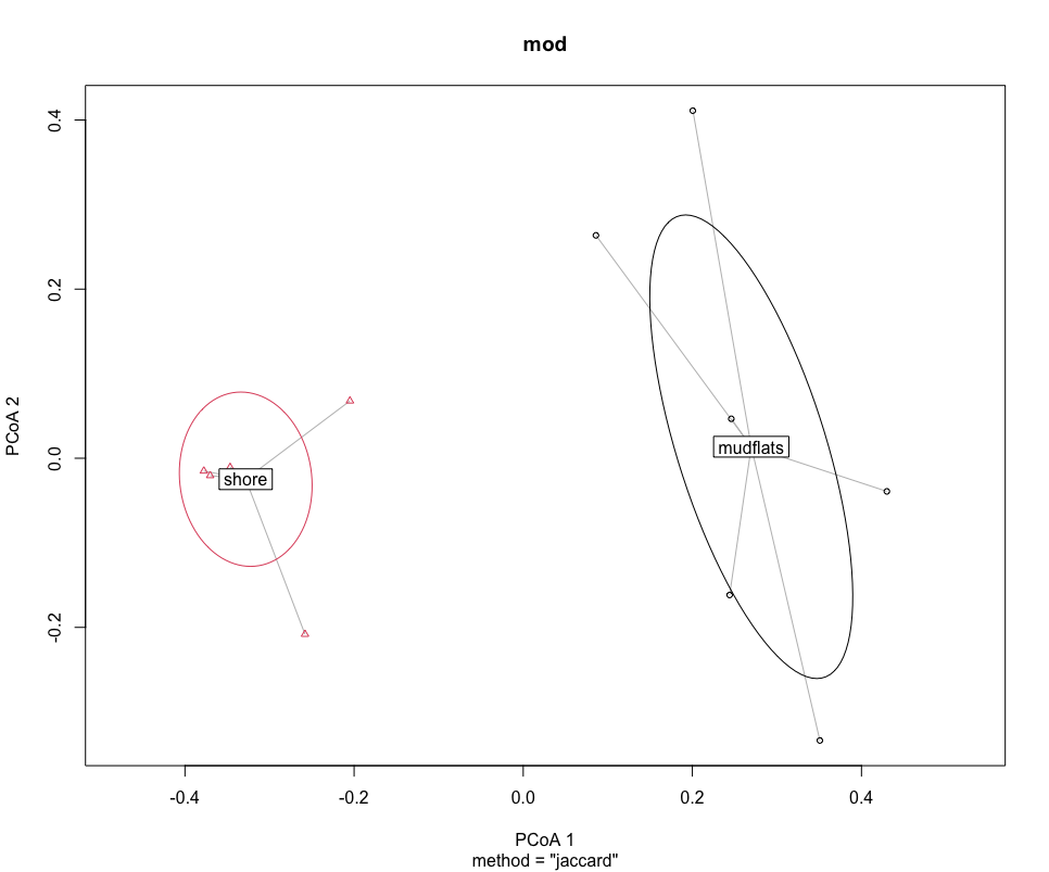
Beta diversity analysis

One final type of analysis we will cover in today’s workshop is in how to determine differences in species composition between sampling locations, i.e., beta diversity analysis. Similar to the alpha diversity analysis, we’ll be working with a presence-absence transformed dataset.

Before we run the statistical analysis, we can visualise differences in species composition through ordination.

#############################
## BETA DIVERSITY ANALYSIS ##
#############################
## transpose dataframe
merged_pa_t <- t(merged_pa)
dis <- vegdist(merged_pa_t, method = 'jaccard')
groups <- factor(c(rep(1,6), rep(2,5)), labels = c('mudflats', 'shore'))
dis
groups
mod <- betadisper(dis, groups)
mod

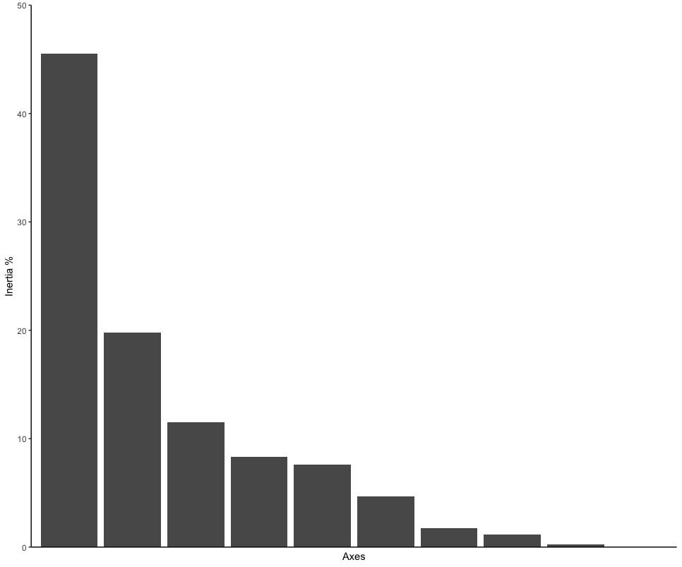
## graph ordination plot and eigenvalues
plot(mod, hull = FALSE, ellipse = TRUE)
ordination_mds <- wcmdscale(dis, eig = TRUE)
ordination_eigen <- ordination_mds$eig
ordination_eigenvalue <- ordination_eigen/sum(ordination_eigen)
ordination_eigen_frame <- data.frame(Inertia = ordination_eigenvalue*100, Axes = c(1:10))
eigenplot <- ggplot(data = ordination_eigen_frame, aes(x = factor(Axes), y = Inertia)) +
  geom_bar(stat = "identity") +
  scale_y_continuous(expand = c(0,0), limits = c(0, 50)) +
  theme_classic() +
  xlab("Axes") +
  ylab("Inertia %") +
  theme(axis.ticks.x = element_blank(), axis.text.x = element_blank())
eigenplot

Next, we can run the statistical analysis PERMANOVA to determine if the sampling locations are significantly different. A PERMANOVA analysis will give a significant result when (i) the centroids of the two sampling locations are different and (ii) if the dispersion of samples to the centroid within a sampling location are different to the other sampling location.

source <- adonis(merged_pa_t ~ Location, data = meta, by = 'terms')
print(source$aov.tab)

Since PERMANOVA can give significant p-values in both instances, we can run an additional test that only provides a significant p-value if the dispersion of samples to the centroid are different between locations.

## test for dispersion effect
boxplot(mod)
set.seed(25)
permutest(mod)

A final test we will cover today, is to determine which taxa are driving the difference in species composition observed during the PERMANOVA and ordination analyses. To accomplish this, we will calculate indicator values for each taxon and identify differences based on IndValij = Specificityij * Fidelityij * 100.

## determine signals driving difference between sampling locations
specrich$Group <- c(1,1,1,1,1,1,2,2,2,2,2)
ISA <- indval(merged_pa_t, clustering = as.numeric(specrich$Group))
summary(ISA)

That is all for the OBSS 2022 eDNA workshop. Thank you all for your participation. Please feel free to contact me for any questions (gjeunen@gmail.com)!

Key Points

• A basic tutorial to conduct statistical analyses of your data