Demultiplexing and Trimming
Overview
Teaching: 20 min
Exercises: 10 minQuestions
What are the different primer design methods for metabarcoding?
How do we demultiplex and quality control metabarcoding data?
Objectives
Learn the different methods for QC of metabarcoding data
Initial processing of raw sequence data
Introduction
To start, let’s navigate to the raw sequencing file in the raw folder within the ~/obss_2021/edna/ directory and list the files in the subdirectory.
$ cd ~/obss_2021/edna/raw/
$ pwd
/home/username/obss_2022/edna/raw
$ ls -ltr
-rwxr-x--- 1 gjeunen staff 124306274 16 Nov 12:39 FTP103_S1_L001_R1_001.fastq.gz
From the output, we can see that we have a single fastq file, the R1_001.fastq.gz file, indicating that the library was sequenced single-end. Therefore, we do not need to merge or assemble paired reads (see Introduction for more information). From the output, we can also see that the sequencing file is currently zipped. This is done to reduce file sizes and facilitate file transfer between the sequencing service and the customer. Most software will be able to read and use zipped files, so there is no need to unzip the file now. However, always check if this is the case when using new software.
Quality control
The first thing we will do with our sequencing file is to look at the quality and make sure everything is according to the sequencing parameters that were chosen. The program we will be using for this is FastQC (EMP). However, since you’ve already encountered this software program, we’ll just focus on the output for now.
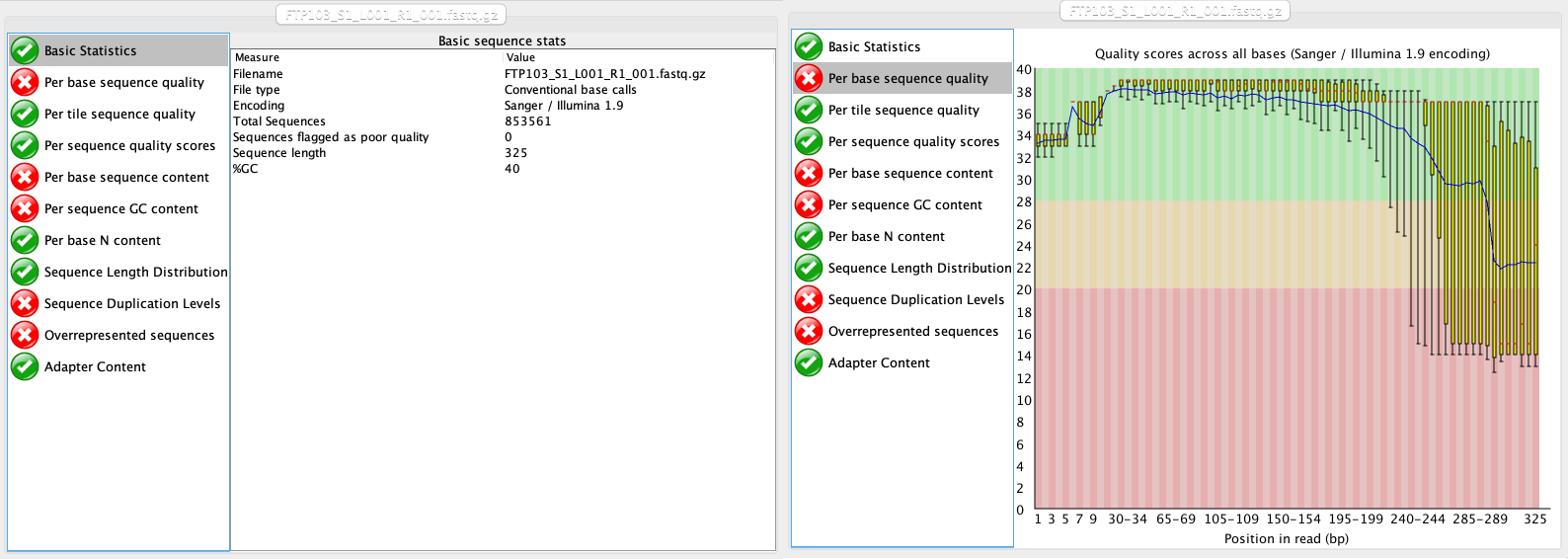
At this stage, we will be looking at the tabs Basic Statistics and Per base sequence quality. From this report, we can see that:
- We have a total of 853,561 sequences.
- The sequence length is 325 bp, identical to the cycle number of the specified sequencing kit.
- Sequence quality is dropping significantly at the end, which is typical for Illumina sequencing data.
Demultiplexing sequencing data
Introduction to demultiplexing
Given that we only have a single sequence file containing all reads for multiple samples, the first step in our pipeline will be to assign each sequence to a sample, a process referred to as demultiplexing. To understand this step in the pipeline, we will need to provide some background on library preparation methods.
As of the time of writing this workshop, PCR amplification is the main method to generate eDNA metabarcoding libraries. To achieve species detection from environmental or bulk specimen samples, PCR amplification is carried out with primers designed to target a taxonomically informative marker within a taxonomic group. Furthermore, next generation sequencing data generates millions of sequences in a single sequencing run. Therefore, multiple samples can be combined. To achieve this, a unique sequence combination is added to the amplicons of each sample. This unique sequence combination is usually between 6 and 8 base pairs long and is referred to as ‘tag’, ‘index’, or ‘barcode’. Besides amplifying the DNA and adding the unique barcodes, sequencing primers and adapters need to be incorporated into the library to allow the DNA to be sequenced by the sequencing machine. How barcodes, sequencing primers, and adapters are added, and in which order they are added to your sequences will influence the data files you will receive from the sequencing service.
For example, traditionally prepared Illumina libraries (ligation and two-step PCR) are constructed in the following manner (the colours mentioned refer to the figure below):
- Forward Illumina adapter (red)
- Forward barcode sequence (darkgreen)
- Forward Illumina sequencing primer (orange)
- Amplicon (including primers)
- Reverse Illumina sequencing primer (lightblue)
- Reverse barcode sequence (lightgreen)
- Reverse Illumina adapter (darkblue)
This construction allows the Illumina software to identify the barcode sequences, which will result in the generation of a separate sequence file (or two for paired-end sequencing data) for each sample. This process is referred to as demultiplexing and is performed by the Illumina software.
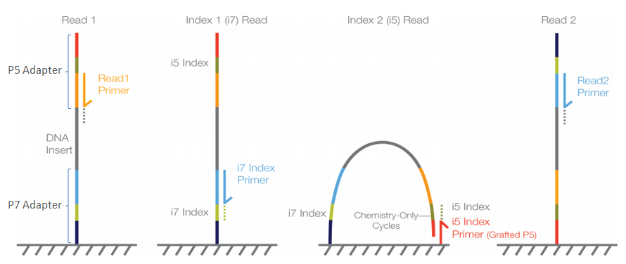
When libraries are prepared using the single-step PCR method, the libraries are constructed slightly different (the colours mentioned refer to the setup described in the two-step approach):
- Forward Illumina adapter (red)
- Forward Illumina sequencing primer (orange)
- Forward barcode sequence (darkgreen)
- Amplicon (including primers)
- Reverse barcode sequence (lightgreen)
- Reverse Illumina sequencing primer (lightblue)
- Reverse Illumina adapter (darkblue)
In this construction, the barcode sequences are not located in between the Illumina adapter and Illumina sequencing primer, but are said to be ‘inline’. These inline barcode sequences cannot be identified by the Illumina software, since it does not know when the barcode ends and the primer sequence of the amplicon starts. Therefore, this will result in a single sequence file (or two for paired-end sequencing data) containing the data for all samples together. The demultiplexing step, assigning sequences to a sample, will have to be incorporated into the bioinformatic pipeline, something we will cover now in the workshop.
For more information on Illumina sequencing, you can watch the following 5-minute youtube video (EMP). Notice that the ‘Sample Prep’ method described in the video follows the two-step PCR approach.
Assigning sequences to corresponding samples
During library preparation for our sample data, each sample was assigned a specific barcode combination, with at least 3 basepair differences between each barcode used in the library. By searching for these specific sequences, which are situated at the very beginning and very end of each sequence, we can assign each sequence to the corresponding sample. We will be using cutadapt for demultiplexing our dataset today, as it is the fastest option. Cutadapt requires an additional metadata text file in fasta format. This text file contains information about the sample name and the associated barcode and primer sequences.
Let’s have a look at the metadata file, which can be found in the meta subfolder.
$ cd ../meta/
$ ls -ltr
-rw-r--r--@ 1 gjeunen staff 1139 16 Nov 12:41 sample_metadata.fasta
$ head -10 sample_metadata.fasta
>AM1
GAAGAGGACCCTATGGAGCTTTAGAC;min_overlap=26...AGTTACYHTAGGGATAACAGCGCGACGCTA;min_overlap=30
>AM2
GAAGAGGACCCTATGGAGCTTTAGAC;min_overlap=26...AGTTACYHTAGGGATAACAGCGCGAGTAGA;min_overlap=30
>AM3
GAAGAGGACCCTATGGAGCTTTAGAC;min_overlap=26...AGTTACYHTAGGGATAACAGCGCGAGTCAT;min_overlap=30
>AM4
GAAGAGGACCCTATGGAGCTTTAGAC;min_overlap=26...AGTTACYHTAGGGATAACAGCGCGATAGAT;min_overlap=30
>AM5
GAAGAGGACCCTATGGAGCTTTAGAC;min_overlap=26...AGTTACYHTAGGGATAACAGCGCGATCTGT;min_overlap=30
From the output, we can see that this is a simple two-line fasta format, with the header line containing the sample name info indicated by ”>” and the barcode/primer info on the following line. We can also see that the forward and reverse barcode/primer sequences are split by “…“ and that we specify a minimum overlap between the sequence found in the data file and the metadata file to be the full length of the barcode/primer information.
Count the number of samples in the metadata file
before we get started with our first script, let’s first determine how many samples are included in our experiment.
Hint 1: think about the file structure of the metadata file. Hint 2: a similar line of code can be written to count the number of sequences in a fasta file (which you might have come across before during OBSS2022)
Solution
grep -c "^>" sample_metadata.fasta
grepis a command that searches for strings that match a pattern-cis the parameter indicating to count the number of times we find the pattern"^>"is the string we need to match, in this case>. The^indicates that the string needs to occur at the beginning of the line.
Let’s now write our first script to demultiplex our sequence data. First, we’ll navigate to the scripts folder. When listing the files in this folder, we see that a script has already been created, so let’s see what it contains. To read the file, we’ll use the nano function.
$ cd ../scripts/
$ ls -ltr
-rwxrwx--x+ 1 jeuge18p uoo02328 63 Nov 17 13:08 moduleload
$ nano moduleload
#!/bin/bash

module load eDNA/2021.11-gimkl-2020a-Python-3.8.2
Here, we can see that the script starts with what is called a shebang #!, which is to let the computer know how to interpret the script. The following line is specific to NeSI, where we will load the necessary software programs to run our scripts. We will, therefore, add this script to all subsequent scripts to make sure the correct software is available on NeSI.
To exit the script, we can press ctr + X, which will bring us back to the terminal window.
To create a new script to demultiplex our data, we can type the following:
$ nano demux
This command will open the file demux in the nano text editor in the terminal. In here, we can type the following commands:
$ #!/bin/bash
$
$ source moduleload
$
$ cd ../raw/
$
$ cutadapt FTP103_S1_L001_R1_001.fastq.gz -g file:../meta/sample_metadata.fasta -o ../input/{name}.fastq --untrimmed-output untrimmed_FTP103.fastq --no-indels -e 0 --cores=0
We can exit out of the text editor by pressing ctr+X, then type y to save the file, and press enter to save the file as demux. When we list the files in the scripts folder, we can see that this file is now created, but that it is not yet executable (no x in file description).
$ ls -ltr
-rwxrwx--x+ 1 jeuge18p uoo02328  63 Nov 17 13:08 moduleload
-rw-rw----+ 1 jeuge18p uoo02328 210 Nov 17 13:24 demux
To make the script executable, we can use the following code:
$ chmod +x demux
When we now list the files in our scripts folder again, we see that the parameters have changed:
$ ls -ltr
-rwxrwx--x+ 1 jeuge18p uoo02328  63 Nov 17 13:08 moduleload
-rwxrwx--x+ 1 jeuge18p uoo02328 210 Nov 17 13:24 demux
To run the script, we can type:
$ ./demux
Once this script has been executed, it will generate quite a bit of output in the terminal. The most important information, however, can be found at the top, indicating how many sequences could be assigned. The remainder of the output is detailed information for each sample.
This is cutadapt 3.5 with Python 3.8.2
Command line parameters: FTP103_S1_L001_R1_001.fastq.gz -g file:../meta/sample_metadata.fasta -o ../input/{name}.fastq --untrimmed-output untrimmed_FTP103.fastq --no-indels -e 0 --cores=0
Processing reads on 70 cores in single-end mode ...
Done           00:00:07       853,561 reads @   9.3 µs/read;   6.47 M reads/minute
Finished in 7.96 s (9 µs/read; 6.43 M reads/minute).

=== Summary ===

Total reads processed:                 853,561
Reads with adapters:                   128,874 (15.1%)
Reads written (passing filters):       853,561 (100.0%)

Total basepairs processed:   277,407,325 bp
Total written (filtered):    261,599,057 bp (94.3%)
If successfully completed, the script should’ve generated a single fastq file for each sample in the input directory. Let’s list these files and look at the structure of the fastq file:
$ ls -ltr ../input/
-rw-rw----+ 1 jeuge18p uoo02328 5404945 Nov 17 13:31 AM1.fastq
-rw-rw----+ 1 jeuge18p uoo02328 4906020 Nov 17 13:31 AM2.fastq
-rw-rw----+ 1 jeuge18p uoo02328 3944614 Nov 17 13:31 AM3.fastq
-rw-rw----+ 1 jeuge18p uoo02328 5916544 Nov 17 13:31 AM4.fastq
-rw-rw----+ 1 jeuge18p uoo02328 5214931 Nov 17 13:31 AM5.fastq
-rw-rw----+ 1 jeuge18p uoo02328 4067965 Nov 17 13:31 AM6.fastq
-rw-rw----+ 1 jeuge18p uoo02328 4841565 Nov 17 13:31 AS2.fastq
-rw-rw----+ 1 jeuge18p uoo02328 9788430 Nov 17 13:31 AS3.fastq
-rw-rw----+ 1 jeuge18p uoo02328 5290868 Nov 17 13:31 AS4.fastq
-rw-rw----+ 1 jeuge18p uoo02328 5660255 Nov 17 13:31 AS5.fastq
-rw-rw----+ 1 jeuge18p uoo02328 4524100 Nov 17 13:31 AS6.fastq
-rw-rw----+ 1 jeuge18p uoo02328     461 Nov 17 13:31 ASN.fastq
$ head -12 ../input/AM1.fastq
@M02181:93:000000000-D20P3:1:1101:15402:1843 1:N:0:1
GACAGGTAGACCCAACTACAAAGGTCCCCCAATAAGAGGACAAACCAGAGGGACTACTACCCCCATGTCTTTGGTTGGGGCGACCGCGGGGGAAGAAGTAACCCCCACGTGGAACGGGAGCACAACTCCTTGAACTCAGGGCCACAGCTCTAAGAAACAAAATTTTTGACCTTAAGATCCGGCAATGCCGATCAACGGACCG
+
2222E2GFFCFFCEAEF3FFBD32FFEFEEE1FFD55BA1AAEEFFE11AA??FEBGHEGFFGE/F3GFGHH43FHDGCGEC?B@CCCC?C??DDFBF:CFGHGFGFD?E?E?FFDBD.-A.A.BAFFFFFFBBBFFBB/.AADEF?EFFFF///9BBFE..BFFFF;.;FFFB///BBFA-@=AFFFF;-BADBB?-ABD;
@M02181:93:000000000-D20P3:1:1101:16533:1866 1:N:0:1
TTTAGAACAGACCATGTCAGCTACCCCCTTAAACAAGTAGTAATTATTGAACCCCTGTTCCCCTGTCTTTGGTTGGGGCGACCACGGGGAAGAAAAAAACCCCCACGTGGACTGGGAGCACCTTACTCCTACAACTACGAGCCACAGCTCTAATGCGCAGAATTTCTGACCATAAGATCCGGCAAAGCCGATCAACGGACCG
+
GGHCFFBFBB3BA2F5FA55BF5GGEGEEHF55B5ABFB5F55FFBGGB55GEEEFEGFFEFGC1FEFFGBBGH?/??EC/>E/FE???//DFFFFF?CDDFFFCFCF...>DAA...<.<CGHFFGGGH0CB0CFFF?..9@FB.9AFFGFBB09AAB?-/;BFFGB/9F/BFBB/BFFF;BCAF/BAA-@B?/B.-.@DA
@M02181:93:000000000-D20P3:1:1101:18101:1874 1:N:0:1
ACTAGACAACCCACGTCAAACACCCTTACTCTGCTAGGAGAGAACATTGTGGCCCTTGTCTCACCTGTCTTCGGTTGGGGCGACCGCGGAGGACAAAAAGCCTCCATGTGGACTGAAGTAACTATCCTTCACAGCTCAGAGCCGCGGCTCTACGCGACAGAAATTCTGACCAAAAATGATCCGGCACATGCCGATTAACGGAACA
+
BFGBA4F52AEA2A2B2225B2AEEGHFFHHF5BD551331113B3FGDGB??FEGG2FEEGBFFGFGCGHE11FE??//>//<</<///<</CFFB0..<F1FE0G0D000<<AC0<000<DDBC:GGG0C00::C0/00:;-@--9@AFBB.---9--///;F9F//;B/....;//9BBA-9-;.BBBB>-;9A/BAA.999
Renaming sequence headers to incorporate sample names
Before we can continue with the next step in our bioinformatic pipeline, we will need to rename every sequence so that the information of the corresponding sample is incorporated. This will be needed to generate our OTU table at the end of the analysis. Lastly, we can combine all the relabeled files into a single file prior to quality filtering.
$ nano rename
$ #!/bin/bash
$
$ source moduleload
$
$ cd ../input/
$
$ for fq in *.fastq; do vsearch --fastq_filter $fq --relabel $fq. --fastqout rl_$fq; done
$
$ cat rl* > ../output/relabel.fastq
$ chmod +x rename
$ ./rename
Once executed, the script will first rename the sequence headers of each file and store them in a new file per sample. Lastly, we have combinned all relabeled files using the cat command. This combined file can be found in the output folder. Let’s see if it is there and how the sequence headers have been altered:
$ ls -ltr ../output/
-rw-rw----+ 1 jeuge18p uoo02328 54738505 Nov 17 13:51 relabel.fastq
head -12 ../output/relabel.fastq
@AM1.fastq.1
GACAGGTAGACCCAACTACAAAGGTCCCCCAATAAGAGGACAAACCAGAGGGACTACTACCCCCATGTCTTTGGTTGGGGCGACCGCGGGGGAAGAAGTAACCCCCACGTGGAACGGGAGCACAACTCCTTGAACTCAGGGCCACAGCTCTAAGAAACAAAATTTTTGACCTTAAGATCCGGCAATGCCGATCAACGGACCG
+
2222E2GFFCFFCEAEF3FFBD32FFEFEEE1FFD55BA1AAEEFFE11AA??FEBGHEGFFGE/F3GFGHH43FHDGCGEC?B@CCCC?C??DDFBF:CFGHGFGFD?E?E?FFDBD.-A.A.BAFFFFFFBBBFFBB/.AADEF?EFFFF///9BBFE..BFFFF;.;FFFB///BBFA-@=AFFFF;-BADBB?-ABD;
@AM1.fastq.2
TTTAGAACAGACCATGTCAGCTACCCCCTTAAACAAGTAGTAATTATTGAACCCCTGTTCCCCTGTCTTTGGTTGGGGCGACCACGGGGAAGAAAAAAACCCCCACGTGGACTGGGAGCACCTTACTCCTACAACTACGAGCCACAGCTCTAATGCGCAGAATTTCTGACCATAAGATCCGGCAAAGCCGATCAACGGACCG
+
GGHCFFBFBB3BA2F5FA55BF5GGEGEEHF55B5ABFB5F55FFBGGB55GEEEFEGFFEFGC1FEFFGBBGH?/??EC/>E/FE???//DFFFFF?CDDFFFCFCF...>DAA...<.<CGHFFGGGH0CB0CFFF?..9@FB.9AFFGFBB09AAB?-/;BFFGB/9F/BFBB/BFFF;BCAF/BAA-@B?/B.-.@DA
@AM1.fastq.3
ACTAGACAACCCACGTCAAACACCCTTACTCTGCTAGGAGAGAACATTGTGGCCCTTGTCTCACCTGTCTTCGGTTGGGGCGACCGCGGAGGACAAAAAGCCTCCATGTGGACTGAAGTAACTATCCTTCACAGCTCAGAGCCGCGGCTCTACGCGACAGAAATTCTGACCAAAAATGATCCGGCACATGCCGATTAACGGAACA
+
BFGBA4F52AEA2A2B2225B2AEEGHFFHHF5BD551331113B3FGDGB??FEGG2FEEGBFFGFGCGHE11FE??//>//<</<///<</CFFB0..<F1FE0G0D000<<AC0<000<DDBC:GGG0C00::C0/00:;-@--9@AFBB.---9--///;F9F//;B/....;//9BBA-9-;.BBBB>-;9A/BAA.999
Key Points
First key point. Brief Answer to questions. (FIXME)