Nanopore-based sequencing: introduction
Overview
Teaching: 35 min
Exercises: 0 minQuestions
What is nanopore-based sequencing?
Objectives
Understand details of ONT sequencing platforms.
What is this module about?
- Long-read sequencing with the Oxford Nanopore Technologies (ONT) platform.
- WHY?
- recent technology advances have led to a surge in popularly for this platform.
- Huge scope for really exciting (and low cost) science
- Concepts and skills learned here are transferable to other sequencing technologies.
- WHAT?
- Genome assembly
- RNA-seq
- Variant identification (single base & structural)
- Base modification (e.g., methylation)
- Metagenomics
ONT platforms
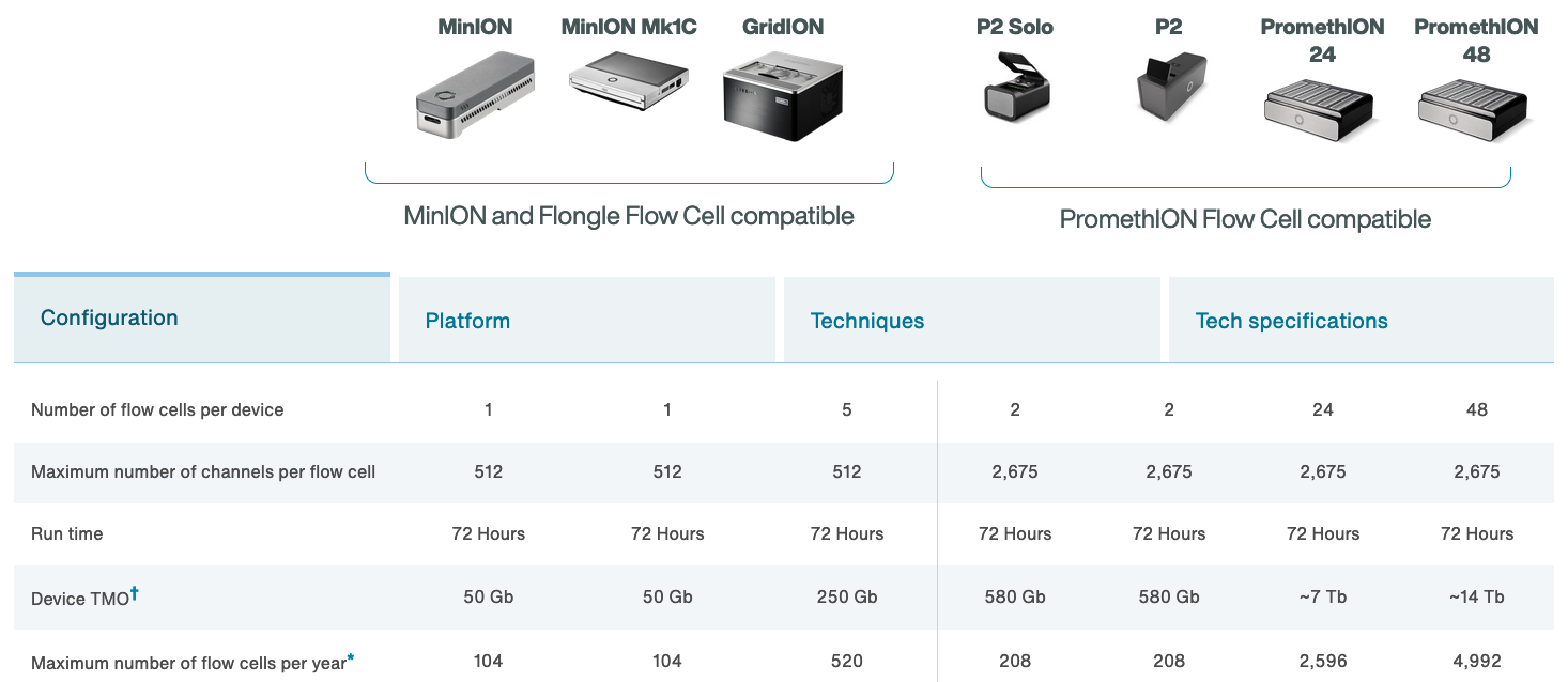
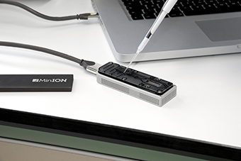
The MinION
http://www.nature.com/news/data-from-pocket-sized-genome-sequencer-unveiled-1.14724
- Rough specs (2014)
- 6-8 hour run time
- sequence per run: ~110Mbp
- average read length: 5,400bp
- reads up to 10kbp
- 2023 specs:
- can run for up to 72 hours
- Maximum (theoretical) yield per run: 50Gbp
- Maximum read length recorded: >4Mbp
https://nanoporetech.com https://nanoporetech.com/products/specifications
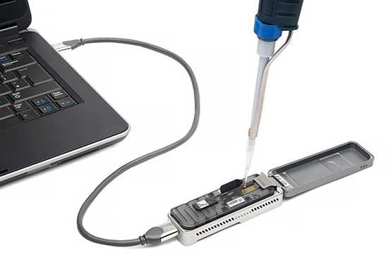
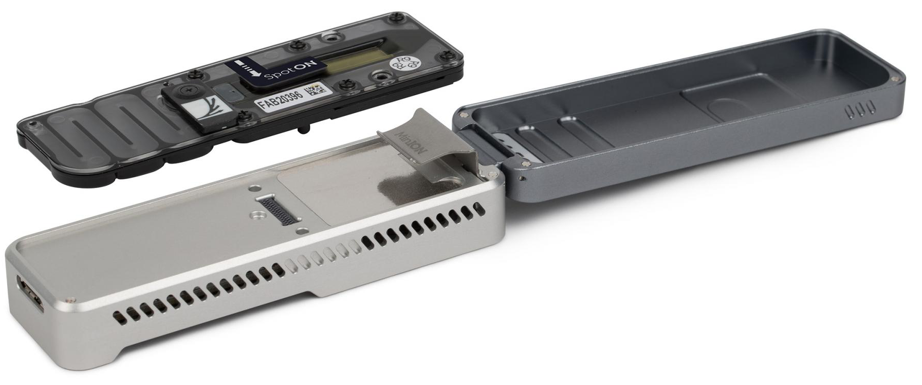
The MinION Mk1B
- The MinION Mk1B is the current version of ONT’s original sequencer.
- Connects to a computer via USB.
https://nanoporetech.com/products/minion
The MinION Mk1C
- The MinION Mk1C provides a truly portable sequencing option, with built in compute and touchscreen.
- For the price, however, the hardware is not particularly impressive.

https://nanoporetech.com/products/minion

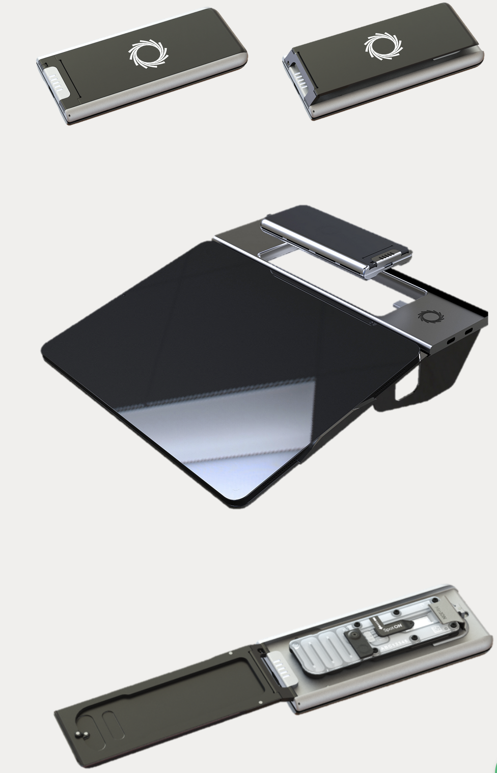
The MinION Mk1D
- The next iteration of portable sequencing devices is the Mk1D.
- Tablet-based (plug-in).
- Currently details are limited, but developer versions
arewere scheduled to be released during 2023: “Further details on specifications will be provided in 2023.”
https://nanoporetech.com/products/minion-mk1d
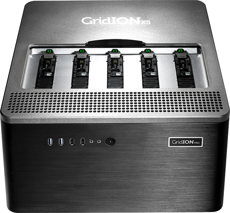
The GridION
- The GridION offers a “medium-throughput” option for Nanopore-based sequencing: can run up to five flowcells at once.
- The MinION (Mk1B and Mk1C) and GridION use the same flow cells
- The Otago Genomics Facility has one of these.
https://nanoporetech.com/products/gridion
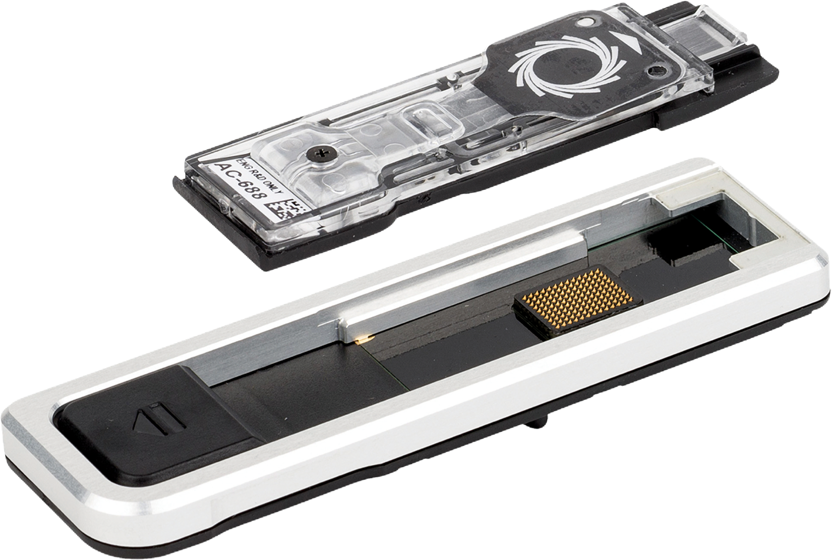
The Flongle
- The Flongle uses an adapter to allow a smaller (and cheaper) flow cell to be used in the MinION and GridION devices.
- Single-use system provides low-cost option for targeted sequencing (e.g., diagnostic applications).
https://nanoporetech.com/products/flongle
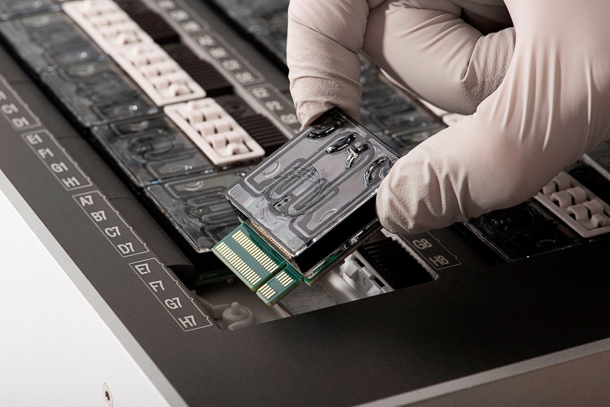
PromethION
- The higher throughout PromethION uses a smaller cartridge-like flow cell. Two options: 24 or 48 flow cells.
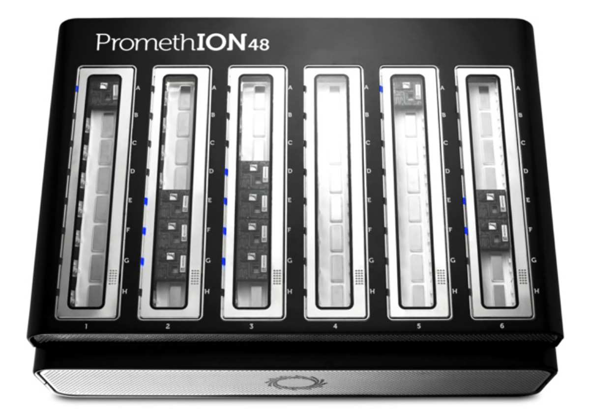
https://nanoporetech.com/products/promethion
A “mini-PromethION”: the P2
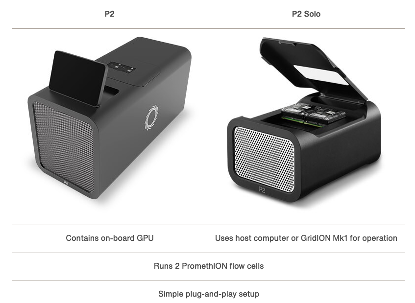
Smaller device (standalone or connect to host computer) that can run Promethion flow cells.
https://nanoporetech.com/products/p2
Flowcell characteristics
- Pores are arranged in sets of four to form a “channel”. Periodically during the sequencing run, the ONT software decides which of the four pores to use from each channel (called a “mux scan”).
- MinION flowcells have 512 channels, so 2048 pores: typically ~1200-1800 are “active” (usable pre-run) (ONT guarantees at least 800 active pores).
- PromethION flowcells have 2675 channels, so 10,700 pores (ONT guarantees at least 5000 active pores).
- Sequencing occurs at roughly 450 bases per second (ONT recommends keeping speed above 300 bases per second - additional reagents can be added to “refuel” the flowcell*), although other speeds are now possible (can prioritise data volume vs accuracy).
-
NOTE: pores are not constantly active, and can become blocked during the run
- https://community.nanoporetech.com/protocols/experiment-companion-minknow/v/mke_1013_v1_revbm_11apr2016/refuelling-your-flow-cell
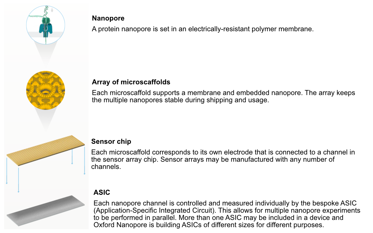
Nanopore technology
https://nanoporetech.com/how-it-works
Nanopore technology
- A motor protein (green) passes a strand of DNA through a nanopore (blue). The current is changed as the bases G, A, T and C pass through the pore in different combinations.
https://nanoporetech.com/how-it-works
Nanopore movies
For more detailed information about ONT sequencing:
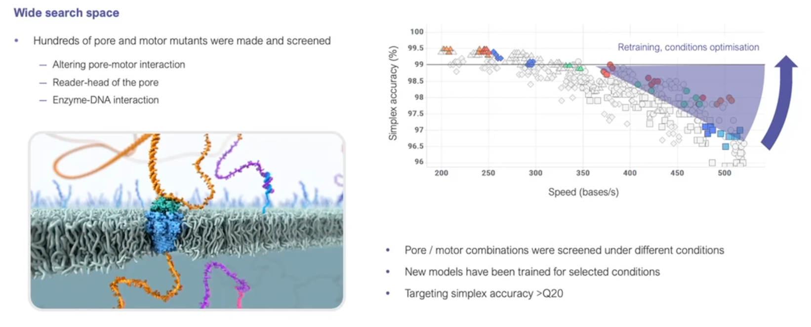
Technological advances…
- Since its introduction, nanopore sequencing has seen a number of improvements.
- The initial product was realtively slow, expensive (per base sequenced) and error prone (i.e., incorrect bases calls).
- Incremental improvements have led to major advances in both speed and accuracy.
https://nanoporetech.com/resource-centre/london-calling-2022-update-oxford-nanopore-technologies
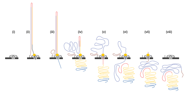
2D sequencing (prior to 2017)
- Hairpin-based approach provided natural error detection methodology:
- Link DNA strands with a hairpin adapter.
- Sequence template strand followed by complement.
- Basecall and compare sequences to produce consensus.
Jain, et al. The Oxford Nanopore MinION: delivery of nanopore sequencing to the genomics community. Genome Biol 17, 239 (2016). https://doi.org/10.1186/s13059-016-1103-0
What happened to 2D reads?
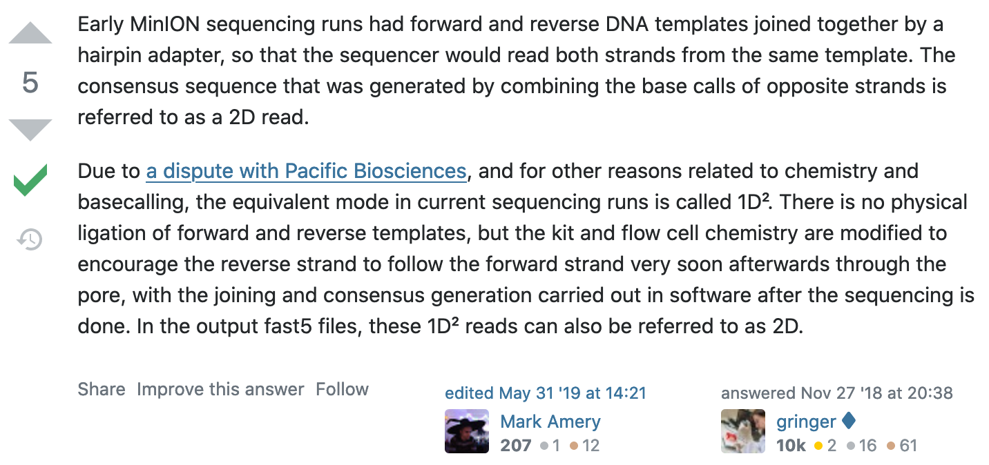
https://bioinformatics.stackexchange.com/questions/5525/what-are-2d-reads-in-the-oxford-minion/5528
The hairpin lawsuit…
- PacBio (competitor in the long-read space) and ONT have filed a number of lawsuits against each other over the past few years.

https://www.genomeweb.com/sequencing/pacbio-oxford-nanopore-settle-patent-dispute-europe
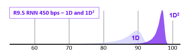
1D2 sequencing
- In 2017 ONT announced the new 1D2 chemistry
- Showed higher accuracy that 1D (and SAID it was better than 2D)
- It didn’t last long…
- Video at link below:
https://nanoporetech.com/about-us/news/1d-squared-kit-available-store-boost-accuracy-simple-prep
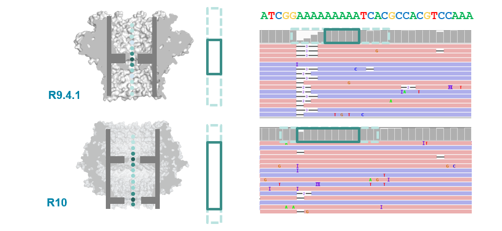
Pore imporvements: the R10 pore
- ONT introduced the new R10 pore in 2019 (previous was R9.4.1).
- Main differences were longer barrel and dual reader head: gave improved resolution of homopolymer runs.
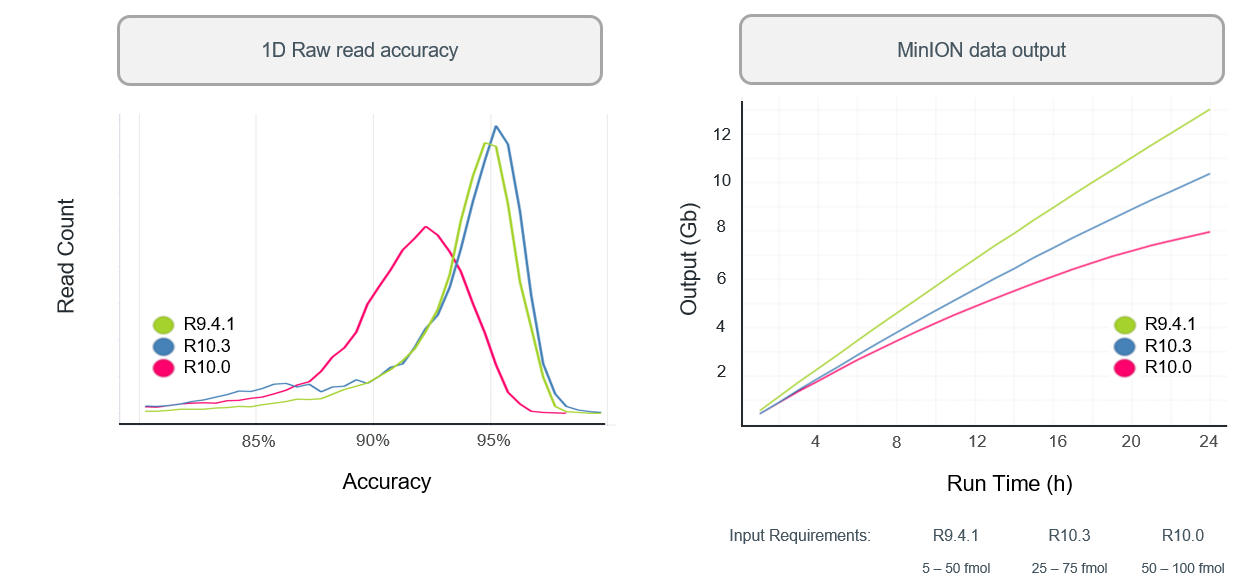
R10.3 vs R9.4.1 performance
- With a bit more tweaking (to get to R10.3) ONT improved 1D (i.e., single-strand) sequencing accuracy, although throughput is still not as high as the R.9.4.1 pore.
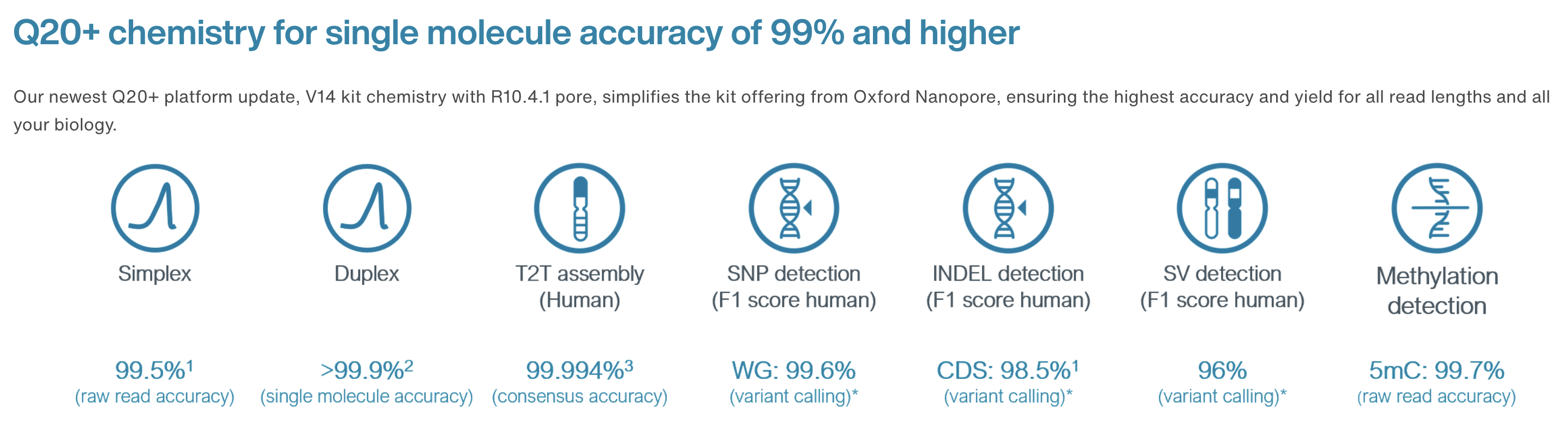
Q20+: the return of 2D reads…
- The previous ONT products are “Q10” (we’ll discuss this soon), meaning that the error rate is roughly 1 incorrect base call per 10 bases (that’s high!)
- The new “Q20+” products are now available - moves to less than 1 error per 100 bases (a little more respectable, but still well below short-read technologies like Illumina).
- Upgrade includes a return to the “2D” approach.

Nanopore workflow
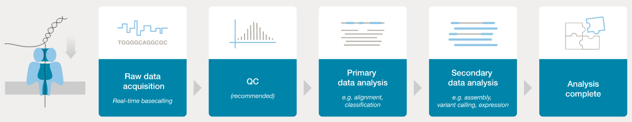
- ONT provides software (MinKNOW) for operating the MinION, and for generating the sequence data (e.g., the
guppyanddoradobasecallers). - Once the raw (POD5 or FAST5 - see next section) data have been converted to basecalls, we can use more familiar tools for quality assessment and analysis (e.g., FastQC).
https://nanoporetech.com/nanopore-sequencing-data-analysis
Basecalling: guppy (deprecated)
guppyis a neural network based basecaller.- analyses the electrical trace data and predicts base
- it is GPU-aware, and can basecall in real time
- can also call base modifications (e.g., 5mC, 6mA)
- high accuracy (HAC) mode (slower) and super-high accuracy (SUP) mode (even slower) can improve basecalls post-sequencing
- MANY other machine learning basecallers have been proposed.
- Output is the standard “FASTQ” format for sequence data.
guppyhas now been “retired” by ONT, and replaced withdorado.
Basecalling: dorado
- ONT has recently released a new base caller:
dorado - Optimised for 10.4.1 flowcells (but there are basecalling models for 9.4.1)
- Designed to support Apple GPUs (M1/M2/M3)
- Like Guppy, can call base modifications
- Also has FAST, HAC and SUP modes for basecalling.
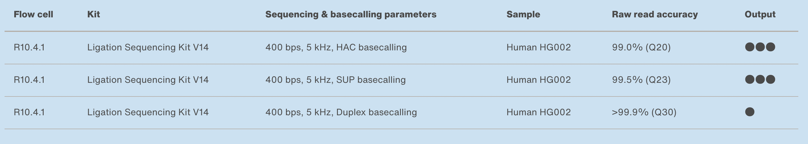
10.4.1 flowcells + v14 chemistry: accuracy
https://nanoporetech.com/accuracy
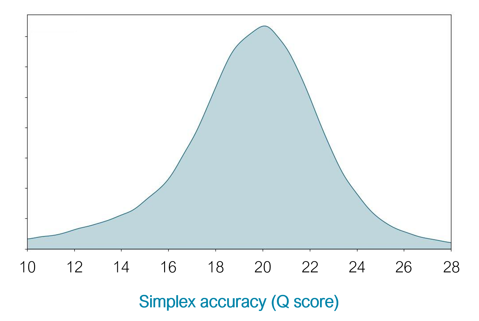
10.4.1 flowcells + v14 chemistry: simplex
- The new chemistry (v14) and updated flowcells (10.4.1) have moved the quality up to ON AVERAGE 1 error per 100 bases (Q20) for simplex reads (single strand).
https://nanoporetech.com/q20plus-chemistry
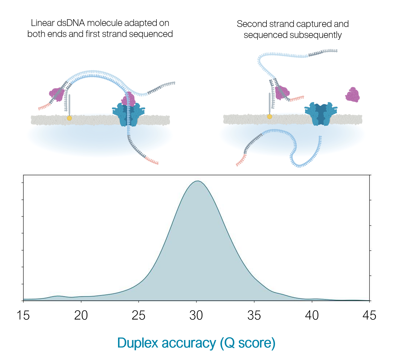
10.4.1 flowcells + v14 chemistry: duplex
- The quality is even higher for duplex reads: mean of 30
- BUT: less than 50% of reads are duplex (i.e., you don’t always manage to read both strands)
https://nanoporetech.com/q20plus-chemistry
More Nanopore: London Calling 2023

- Online conference held in May 2023
- Talk videos available online
- LOTS of really cool announcements and research applications
- Can also watch presentations from previous years.
Key Points
ONT produce a range of popular sequencing platforms.
This technology is constantly advancing.
Data Transfer
Overview
Teaching: 10 min
Exercises: 0 minQuestions
How do I get data to and from NeSI?
Objectives
Understand how to transfer data with Globus.
Understand how to transfer data with
scp.Understand how to transfer data within JupyterHub.
Up until now all the data that we have used for the Otago Bioinformatics Spring School has been either already on NeSI or able to be downladed there from the internet. With bioinformatics workflows we usually start with needing to get our data from our computer to the computers being used for processing and analysis and then once that is done, we need to transfer it back.
There are three main ways to go about transferring data between your computer and NeSI. These are using scp on the commandline, through the upload/download option when running a Jupyter notebook session on NeSI, or through Globus.
Both scp and Jupyter methods are only really suitable for small data transfers (< 1 GB). For anything larger, it is recommended to use Globus.
Generating FASTQ data - basecalling
During the ONT sequencing run, the electrical trace (“squiggle”) data generated by the flowcell are stored in POD5 format (or FAST5, if using older data). In order to perform further analysis, the POD5 data needs to basecalled. Previously ONT basecalling software (guppy) output to FASTQ format (base calls plus associated quality information), but dorado outputs to (unaligned) .bam format by default (although you can still choose FASTQ by changing the output settings).
Basecalling usually occurs while a sequencing run is underway, but there are some specific situations that will require you to “re-basecall” your data:
-
You didn’t perform any basecalling while sequencing - e.g., a MinION being run from a computer without a GPU (so real-time basecalling not possible)
-
You performed basecalling in FAST mode while sequencing, and now you would like to “re-basecall” using a more accurate model (e.g., super-high accuracy mode: SUP)
You may also have downloaded some POD5 or FAST5 data (i.e., without basecalls), or have access to some older POD5/FAST5 data, and you would like re-basecall using a more recent version of ONT’s software.
In all of these cases, we need to get the POD5/FAST5 data onto a compute system where you have access to a GPU.
Today we will use NeSI for this.
The first step in the process is to transfer our POD5 data to NeSI.
scp
From a terminal, scp can be used to transfer files to a remote computer.
The documentation for how to use scp specifically with NeSI can be found at https://support.nesi.org.nz/hc/en-gb/articles/360000578455-File-Transfer-with-SCP. There are some configuration steps that need to be done to make this a bit easier.
The general format is scp <local file to transfer> mahuika:<path to copy file to> to send a file to NeSI, and scp mahuika:<path to file> <local path to copy to> to copy a file from NeSI to your machine.
Jupyter
Jupyter can be used to both upload and download data, however similar to scp it’s not ideal for sending large quantities of data.
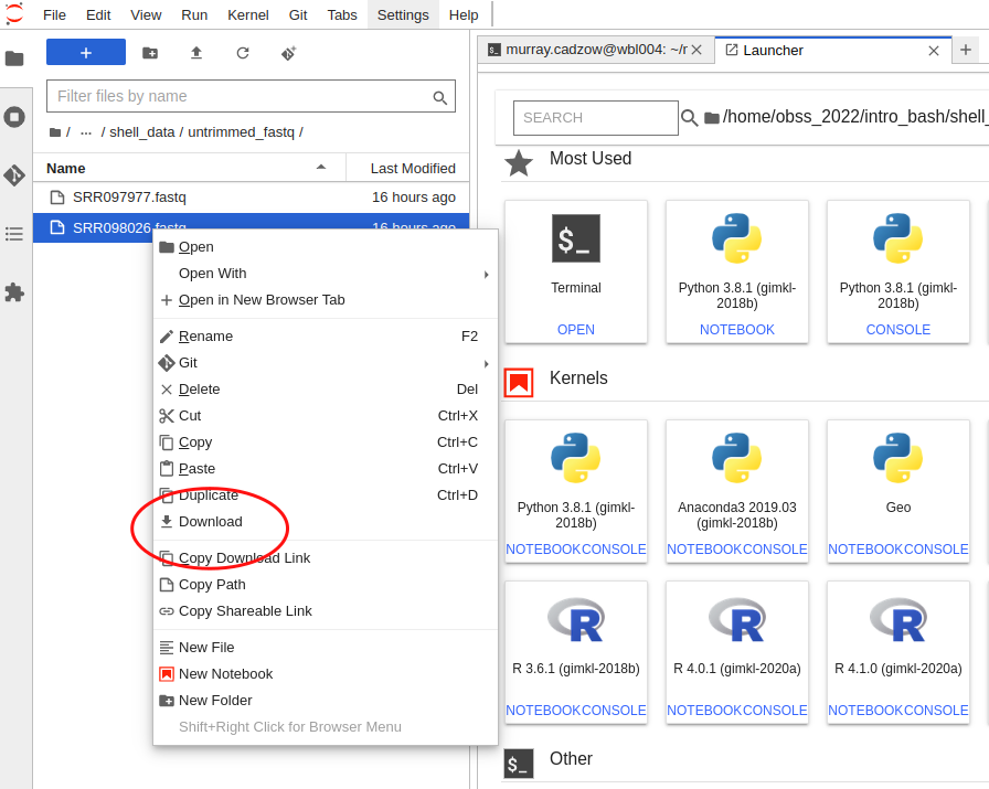
Downloading data
To download a file using Jupyter, you will need to use the explorer panel and navigate to the file there. Then, right-click on th file and a menu will pop up. Select “Download” from this menu and your browser will start downloading it.
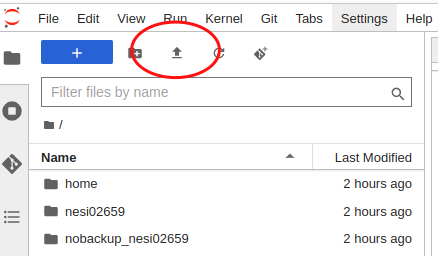
Uploading data
Similar to downloading through Juptyer, you first need to use the explorer panel to navigate to the directory where you would like the file to be uploaded to. From there click the upload button in the top left corner and select the file you wish to upload from your computer.
Globus
Globus is specialised software that can handle the transfer of large amounts of data between two ‘endpoints’. As part of the transfer it can automatically perform the file integrity checks to ensure the file was correctly transferred. The documentation for using Globus with NeSI is found at https://support.nesi.org.nz/hc/en-gb/articles/4405623380751-Data-Transfer-using-Globus-V5.
NeSI provides an endpoint, and you need to provide the second - this might be the globus software running on a different server, or the globus software running on your computer.
Globus Personal Connect
If you need to transfer data from your own machine, you can create your own endpoint by installing and running the Globus Personal Connect software avaiable from https://www.globus.org/globus-connect-personal.
Key Points
There are multiple methods to transfer data to and from NeSI.
The method of choice depends on the size of the data.
Nanopore - Basecalling
Overview
Teaching: 30 min
Exercises: 30 minQuestions
How do you perform offline (i.e., non-live) basecalling for ONT data?
Objectives
Understand POD5/FASTQ format.
Use dorado on NeSI to generate basecalled data from POD5 or FAST5 output files.
FAST5 / HDF5 data
- Each pore produces a HUGE amount of data - very roughly, 1Gbp of sequence data requires 1GB of storage (e.g., as gzipped fastq), but to generate 1Gbp of sequence requires 10GB of electrical trace data, so potentially up to 500GB of files for a 72 hour MinION run.
- (Until recently) the electrical trace data was saved as “.fast5”, which utilises the HDF5 file format:
“Hierarchical Data Format (HDF) is a set of file formats (HDF4, HDF5) designed to store and organize large amounts of data. Originally developed at the National Center for Supercomputing Applications, it is supported by The HDF Group, a non-profit corporation whose mission is to ensure continued development of HDF5 technologies and the continued accessibility of data stored in HDF.”
https://www.neonscience.org/resources/learning-hub/tutorials/about-hdf5
POD5 format
- Over the past year (or so) ONT have introduced the POD5 format for storing data.
- This is a more efficient file format (e.g., faster read and write, smaller) than FAST5.
- New ONT tools (e.g., the dorado basecaller) can process POD5 data.
- ONT offers tools (online and Python-based) for converting between FAST5 and POD5:
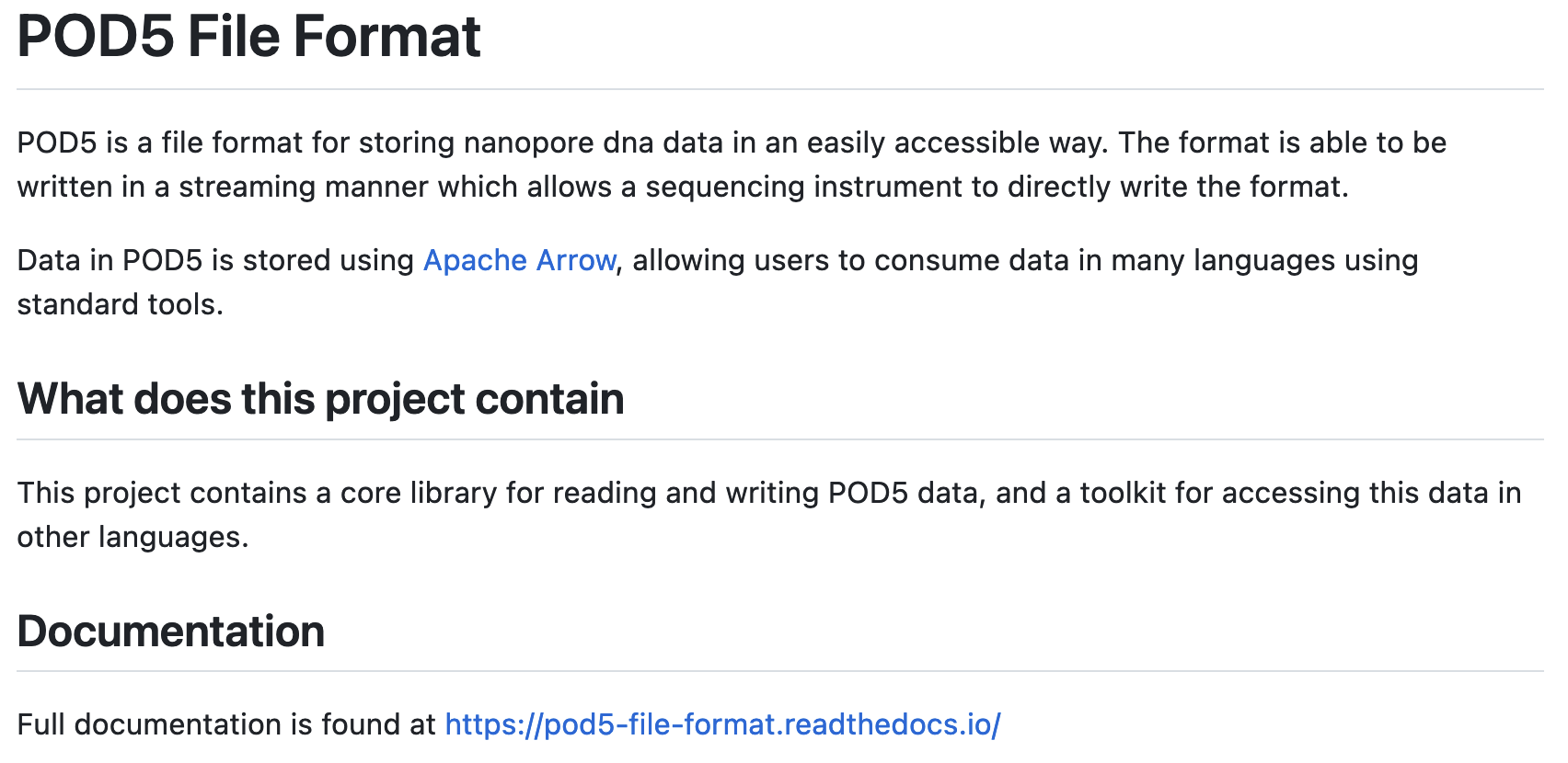
https://pod5.nanoporetech.com/
Basecalling workflow
In order to analyse the data from a sequencing run, the POD5/FAST5 “squiggle” data needs to be converted to base calls.
The ONT software application dorado can be used to process POD5/FAST5 data and generate basecalls and quality information.
Previously this was outoput as FASTQ - a widely used format for storage of sequence data and associated base-level quality scores. This same information is now stored in (unaligned) BAM format (BAM is a binary version of SAM format, which was created for storing aligment information, along with sequence data and quality scores for reads, but it can also be used to stored unaligned data: basecalls and quality scores).
- ONT provides software (MinKNOW) for operating the MinION, and for generating the sequence data (e.g., the
doradobasecaller). - Once the raw data have been converted to basecalls, we can use more familiar tools for quality assessment and analysis (e.g., FastQC).
https://nanoporetech.com/nanopore-sequencing-data-analysis
The current version of the dorado software can be downloaded from GitHub:
https://github.com/nanoporetech/dorado
Today we will be using dorado on the NeSI system to generate FASTQ data from a set of POD5 files.
Recap: FASTQ data format
Assessing sequence quality: phred scores
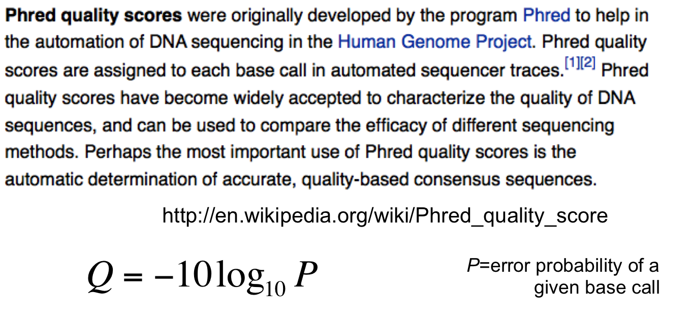
Ewing B, Green P. (1998): Base-calling of automated sequencer traces using phred. II. Error probabilities. Genome Res. 8(3):186-194.
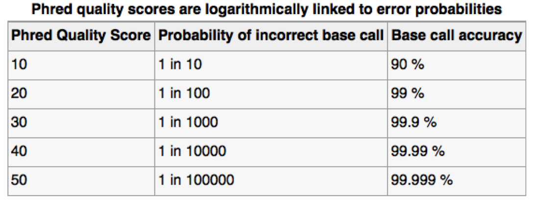
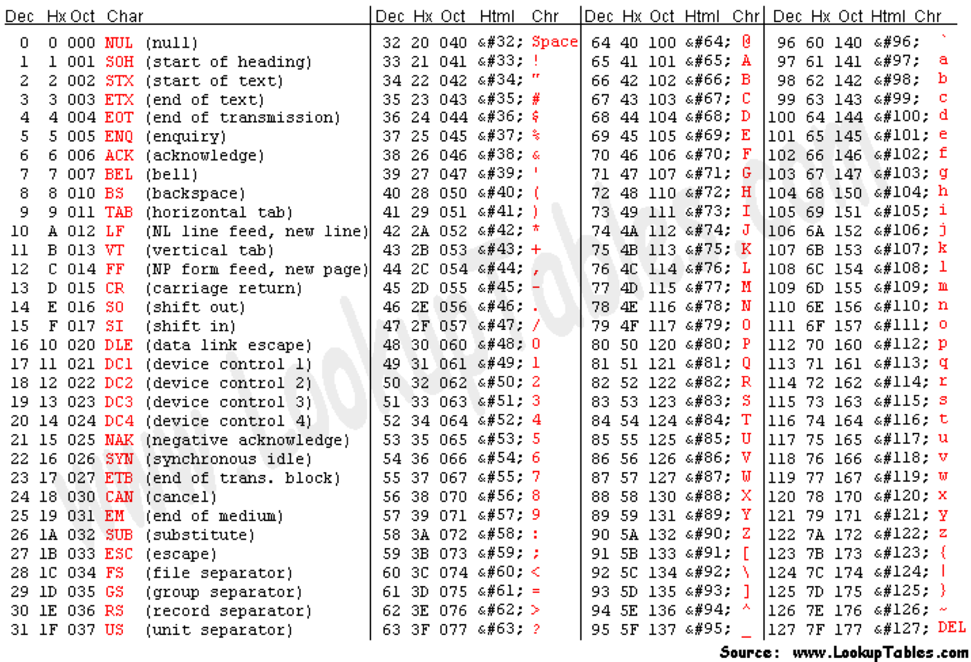
Can use ASCII to represent quality scores by adding 33 to the phred score and converting to ASCII.
- Quality score of 38 becomes 38+33=71: “G”
http://en.wikipedia.org/wiki/Phred_quality_score
- The FASTQ format allows the storage of both sequence and quality information for each read.
- This is a compact text-based format that has become the de facto standard for storing data from next generation sequencing experiments.
FASTQ format:
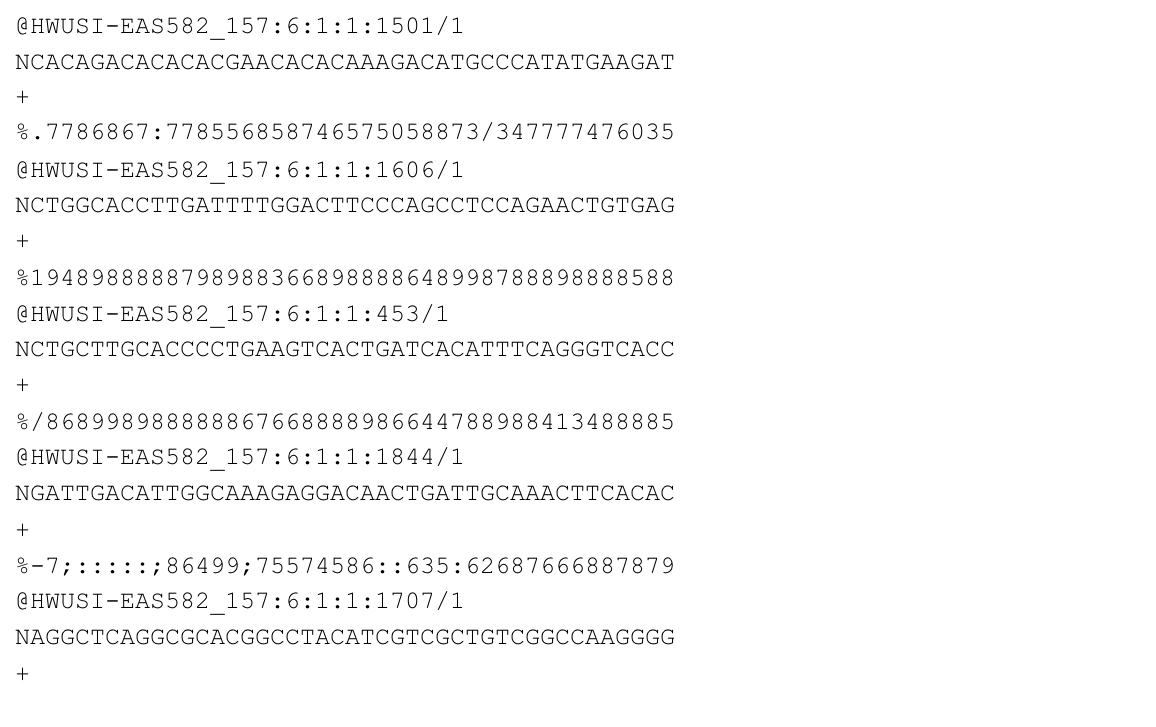
http://en.wikipedia.org/wiki/FASTQ_format
- Line 1: ‘@’ character followed by sequence identifier and optional description.
- Line 2: base calls.
- Line 3: ‘+’ character, optionally followed by the same sequence identifier (and description) again.
- Line 4: quality scores
BAM instead of FASTQ
dorado outputs sequence and quality information to BAM format by default.
BAM is a binary (compressed) version of the text-based SAM format (warning, not a thrilling read):
https://samtools.github.io/hts-specs/SAMv1.pdf
E coli data set on NeSI
For this part of the workshop we are working at:
~/obss_2023/nanopore/ecoli-data/
Let’s change to that directory now:
cd ~/obss_2023/nanopore/ecoli-data/
POD5 files from sequencing E. coli are available in the directory:
pod5_pass
ls -1 pod5_pass
ecoli_pass_0.pod5
ecoli_pass_10.pod5
ecoli_pass_11.pod5
ecoli_pass_12.pod5
ecoli_pass_14.pod5
ecoli_pass_15.pod5
ecoli_pass_1.pod5
ecoli_pass_2.pod5
ecoli_pass_3.pod5
ecoli_pass_4.pod5
ecoli_pass_5.pod5
ecoli_pass_6.pod5
ecoli_pass_8.pod5
Basecalling: dorado
doradois a neural network based basecaller.- analyses the electrical trace data and predicts base
- it is GPU-aware, and can basecall in real time
- can also call base modifications (e.g., 5mC, 5hmC, 6mA)
- common to use the “fast” basecalling model to generate basecalls and quality scores during sequening run.
- high accuracy mode (HAC: slower) and super-high accuracy mode (SUP: even slower) can improve basecalls post-sequencing
- Output is unaligned BAM format.
On NeSI:
module spider Dorado
------------------------------------------------------------------------------
  Dorado:
------------------------------------------------------------------------------
    Description:
      High-performance, easy-to-use, open source basecaller for Oxford
      Nanopore reads.

     Versions:
        Dorado/0.2.1
        Dorado/0.2.4
        Dorado/0.3.0
        Dorado/0.3.1
        Dorado/0.3.2
        Dorado/0.3.4-rc2
        Dorado/0.3.4
        Dorado/0.4.0
        Dorado/0.4.1
        Dorado/0.4.2
        Dorado/0.4.3

------------------------------------------------------------------------------
  For detailed information about a specific "Dorado" module (including how to load the modules) use the module's full name.
  For example:

     $ module spider Dorado/0.4.3
------------------------------------------------------------------------------
module load Dorado/0.4.3

dorado --help
Usage: dorado [options] subcommand

Positional arguments:
aligner
basecaller
demux
download
duplex
summary

Optional arguments:
-h --help               shows help message and exits
-v --version            prints version information and exits
-vv                     prints verbose version information and exits
Using dorado on NeSI
Information about using dorado on NeSI can be found at:
https://support.nesi.org.nz/hc/en-gb/articles/6623692647951-Dorado
In order to use dorado to generate basecalls from POD5 of FAST5 data, we need to select a “model”.
Each model has been trained to generate specific types of basecalls (i.e., unmodified DNA, RNA, modified DNA: 5mC, 5hmC, 6mA), for specific types of data (flowcell version: 9.4.1, 10.4.1; *plex: simplex, duplex; speed: 260bps, 400bps or 70bps/130bp for RNA), at differing levels of accuracy (FAST, HAC, SUP).
We can see what models are available via:
dorado download --list
[2023-11-26 01:37:39.797] [info] > modification models
[2023-11-26 01:37:39.797] [info]  - dna_r10.4.1_e8.2_260bps_fast@v3.5.2_5mCG@v2
[2023-11-26 01:37:39.797] [info]  - dna_r10.4.1_e8.2_260bps_fast@v4.0.0_5mCG_5hmCG@v2
[2023-11-26 01:37:39.797] [info]  - dna_r10.4.1_e8.2_260bps_fast@v4.1.0_5mCG_5hmCG@v2
[2023-11-26 01:37:39.797] [info]  - dna_r10.4.1_e8.2_260bps_hac@v3.5.2_5mCG@v2
[2023-11-26 01:37:39.797] [info]  - dna_r10.4.1_e8.2_260bps_hac@v4.0.0_5mCG_5hmCG@v2
[2023-11-26 01:37:39.797] [info]  - dna_r10.4.1_e8.2_260bps_hac@v4.1.0_5mCG_5hmCG@v2
[2023-11-26 01:37:39.797] [info]  - dna_r10.4.1_e8.2_260bps_sup@v3.5.2_5mCG@v2
[2023-11-26 01:37:39.797] [info]  - dna_r10.4.1_e8.2_260bps_sup@v4.0.0_5mCG_5hmCG@v2
[2023-11-26 01:37:39.797] [info]  - dna_r10.4.1_e8.2_260bps_sup@v4.1.0_5mCG_5hmCG@v2
[2023-11-26 01:37:39.797] [info]  - dna_r10.4.1_e8.2_400bps_fast@v3.5.2_5mCG@v2
[2023-11-26 01:37:39.797] [info]  - dna_r10.4.1_e8.2_400bps_fast@v4.0.0_5mCG_5hmCG@v2
[2023-11-26 01:37:39.797] [info]  - dna_r10.4.1_e8.2_400bps_fast@v4.1.0_5mCG_5hmCG@v2
[2023-11-26 01:37:39.797] [info]  - dna_r10.4.1_e8.2_400bps_fast@v4.2.0_5mCG_5hmCG@v2
[2023-11-26 01:37:39.797] [info]  - dna_r10.4.1_e8.2_400bps_hac@v3.5.2_5mCG@v2
[2023-11-26 01:37:39.797] [info]  - dna_r10.4.1_e8.2_400bps_hac@v4.0.0_5mCG_5hmCG@v2
[2023-11-26 01:37:39.797] [info]  - dna_r10.4.1_e8.2_400bps_hac@v4.1.0_5mCG_5hmCG@v2
[2023-11-26 01:37:39.797] [info]  - dna_r10.4.1_e8.2_400bps_hac@v4.2.0_5mCG_5hmCG@v2
[2023-11-26 01:37:39.797] [info]  - dna_r10.4.1_e8.2_400bps_sup@v3.5.2_5mCG@v2
[2023-11-26 01:37:39.797] [info]  - dna_r10.4.1_e8.2_400bps_sup@v4.0.0_5mCG_5hmCG@v2
[2023-11-26 01:37:39.797] [info]  - dna_r10.4.1_e8.2_400bps_sup@v4.1.0_5mCG_5hmCG@v2
[2023-11-26 01:37:39.797] [info]  - dna_r10.4.1_e8.2_400bps_sup@v4.2.0_5mC@v2
[2023-11-26 01:37:39.798] [info]  - dna_r10.4.1_e8.2_400bps_sup@v4.2.0_5mCG_5hmCG@v2
[2023-11-26 01:37:39.798] [info]  - dna_r10.4.1_e8.2_400bps_sup@v4.2.0_5mCG_5hmCG@v3.1
[2023-11-26 01:37:39.798] [info]  - dna_r10.4.1_e8.2_400bps_sup@v4.2.0_5mC_5hmC@v1
[2023-11-26 01:37:39.798] [info]  - dna_r10.4.1_e8.2_400bps_sup@v4.2.0_6mA@v2
[2023-11-26 01:37:39.798] [info]  - dna_r10.4.1_e8.2_400bps_sup@v4.2.0_6mA@v3
[2023-11-26 01:37:39.798] [info]  - dna_r9.4.1_e8_fast@v3.4_5mCG@v0.1
[2023-11-26 01:37:39.798] [info]  - dna_r9.4.1_e8_fast@v3.4_5mCG_5hmCG@v0
[2023-11-26 01:37:39.798] [info]  - dna_r9.4.1_e8_hac@v3.3_5mCG@v0.1
[2023-11-26 01:37:39.798] [info]  - dna_r9.4.1_e8_hac@v3.3_5mCG_5hmCG@v0
[2023-11-26 01:37:39.798] [info]  - dna_r9.4.1_e8_sup@v3.3_5mCG@v0.1
[2023-11-26 01:37:39.798] [info]  - dna_r9.4.1_e8_sup@v3.3_5mCG_5hmCG@v0
[2023-11-26 01:37:39.798] [info]  - rna004_130bps_sup@v3.0.1_m6A_DRACH@v1
[2023-11-26 01:37:39.798] [info] > stereo models
[2023-11-26 01:37:39.798] [info]  - dna_r10.4.1_e8.2_4khz_stereo@v1.1
[2023-11-26 01:37:39.798] [info]  - dna_r10.4.1_e8.2_5khz_stereo@v1.1
[2023-11-26 01:37:39.798] [info] > simplex models
[2023-11-26 01:37:39.798] [info]  - dna_r10.4.1_e8.2_260bps_fast@v3.5.2
[2023-11-26 01:37:39.798] [info]  - dna_r10.4.1_e8.2_260bps_fast@v4.0.0
[2023-11-26 01:37:39.798] [info]  - dna_r10.4.1_e8.2_260bps_fast@v4.1.0
[2023-11-26 01:37:39.798] [info]  - dna_r10.4.1_e8.2_260bps_hac@v3.5.2
[2023-11-26 01:37:39.798] [info]  - dna_r10.4.1_e8.2_260bps_hac@v4.0.0
[2023-11-26 01:37:39.798] [info]  - dna_r10.4.1_e8.2_260bps_hac@v4.1.0
[2023-11-26 01:37:39.798] [info]  - dna_r10.4.1_e8.2_260bps_sup@v3.5.2
[2023-11-26 01:37:39.798] [info]  - dna_r10.4.1_e8.2_260bps_sup@v4.0.0
[2023-11-26 01:37:39.798] [info]  - dna_r10.4.1_e8.2_260bps_sup@v4.1.0
[2023-11-26 01:37:39.798] [info]  - dna_r10.4.1_e8.2_400bps_fast@v3.5.2
[2023-11-26 01:37:39.798] [info]  - dna_r10.4.1_e8.2_400bps_fast@v4.0.0
[2023-11-26 01:37:39.798] [info]  - dna_r10.4.1_e8.2_400bps_fast@v4.1.0
[2023-11-26 01:37:39.798] [info]  - dna_r10.4.1_e8.2_400bps_fast@v4.2.0
[2023-11-26 01:37:39.798] [info]  - dna_r10.4.1_e8.2_400bps_hac@v3.5.2
[2023-11-26 01:37:39.798] [info]  - dna_r10.4.1_e8.2_400bps_hac@v4.0.0
[2023-11-26 01:37:39.798] [info]  - dna_r10.4.1_e8.2_400bps_hac@v4.1.0
[2023-11-26 01:37:39.798] [info]  - dna_r10.4.1_e8.2_400bps_hac@v4.2.0
[2023-11-26 01:37:39.798] [info]  - dna_r10.4.1_e8.2_400bps_sup@v3.5.2
[2023-11-26 01:37:39.798] [info]  - dna_r10.4.1_e8.2_400bps_sup@v4.0.0
[2023-11-26 01:37:39.798] [info]  - dna_r10.4.1_e8.2_400bps_sup@v4.1.0
[2023-11-26 01:37:39.798] [info]  - dna_r10.4.1_e8.2_400bps_sup@v4.2.0
[2023-11-26 01:37:39.798] [info]  - dna_r9.4.1_e8_fast@v3.4
[2023-11-26 01:37:39.798] [info]  - dna_r9.4.1_e8_hac@v3.3
[2023-11-26 01:37:39.798] [info]  - dna_r9.4.1_e8_sup@v3.3
[2023-11-26 01:37:39.798] [info]  - dna_r9.4.1_e8_sup@v3.6
[2023-11-26 01:37:39.798] [info]  - rna002_70bps_fast@v3
[2023-11-26 01:37:39.798] [info]  - rna002_70bps_hac@v3
[2023-11-26 01:37:39.799] [info]  - rna004_130bps_fast@v3.0.1
[2023-11-26 01:37:39.799] [info]  - rna004_130bps_hac@v3.0.1
[2023-11-26 01:37:39.799] [info]  - rna004_130bps_sup@v3.0.1
We can ask dorado to download a specific model via:
mkdir dorado-models
dorado download --model dna_r9.4.1_e8_fast@v3.4 --directory dorado-models/
dorado can use GPUs to speed up the basecalling process.
On NeSI, we can access the A100 GPUs by submitting a job to the cluster using a slurm script.
The slurm script we will use can be found at:
scripts/dorado_fastmodel.sl
Let’s have a look at the content:
more scripts/dorado_fastmodel.sl
#!/bin/bash -e

#SBATCH --job-name      dorado_basecalling
#SBATCH --time          00:10:00
#SBATCH --mem           6G
#SBATCH --cpus-per-task 4
#SBATCH --output        dorado_%j.out
#SBATCH --account       nesi02659
#SBATCH --gpus-per-node A100-1g.5gb:1

module purge
module load Dorado/0.4.3

dorado download --model dna_r9.4.1_e8_fast@v3.4 --directory dorado-models/

dorado basecaller  --device 'cuda:all' dorado-models/dna_r9.4.1_e8_fast@v3.4 pod5_pass/ > bam-unaligned/ecoli-pod5-pass-basecalls.bam
- The
SBATCHcommands are providing information to theslurmjob scheduler: job name, maximum run time, memory allocation etc - The
modulecommands are making sure the necessary modules are available to the script (here we are specifying version 0.4.3 ofDorado- the GPU-enabled version of ONT’s dorado software). - The
dorado downloadcommand downloads the model that we want to use for basecalling, and saves it to thedorado-modelsdirectory. - The
dorado basecallercommand is what is doing the work (i.e., converting the .pod5 data to unaligned .bam).
Let’s have a closer look at the dorado basecaller command:
dorado basecaller  \
  --device 'cuda:all' \
  dorado-models/dna_r9.4.1_e8_fast@v3.4 \
  pod5_pass \
  > bam-unaligned/ecoli-pod5-pass-basecalls.bam
Options used:
--device 'cuda:all': this refers to which GPU device should be used (here we let the software select useallavailable devices, but it can sometimes be useful to select specific GPU devices).-s fastq_fastmodel: the name of the folder where the .fastq files will be written to.dorado-models/dna_r9.4.1_e8_fast@v3.4: this specifies the model (and its location, relative to wheer we call the script from) that is being used to perform the basecalling. In this case we are using the “fast” model (rather than high-accuracy (hac) or super-high accuracy (sup)) to save time, anddnadenotes that we sequenced… DNA.r9.4.1refers to the flowcell version that was used to generate the data, and e8 is the kit chemistry that was used for library generation (e8 is kit9 or kit 10, e8.2 is kit 14).pod5_pass: this is the directory containing the.pod5(or.fast5-doradowith process either type) files that we would like to process.bam-unaligned/ecoli-pod5-pass-basecalls.bam: output file location (not that the “>” character sends the output fromdoradoto this file).
Before running the script, we need to create the directory where the output files will be written:
mkdir bam-unaligned
To submit the script, we use the sbatch command, and run it from the ~/obss_2023/nanopore/ecoli-data directory. You can check
if you are in that directory with pwd. If not:
cd ~/obss_2023/nanopore/ecoli-data
To run the script:
sbatch scripts/dorado_fastmodel.sl
Once the script has been submitted, you can check to make sure it is running via:
# This shows all your current jobs
squeue --me
JOBID         USER     ACCOUNT   NAME        CPUS MIN_MEM PARTITI START_TIME     TIME_LEFT STATE    NODELIST(REASON)
41491249      michael. nesi02659 dorado_basec   4      6G gpu     2023-11-26T0        8:31 RUNNING  wbl001
41491302      michael. nesi02659 spawner-jupy   4      8G interac 2023-11-26T0       28:44 RUNNING  wbn001
It will also write “progress” output to a log file that contains the job ID (represented by XXXXXXX in the code below), although (unlike with the
older guppy software, you don’t get any information about how far through the processing you are).
You can check the file name using ls -ltr (list file details, in reverse time order).
Using the tail -f command, we can watch the “progress” (use control-c to exit):
ls -ltr
tail -f dorado_XXXXXXX.out
Example of output:
[2023-11-26 02:01:36.919] [info] > Creating basecall pipeline
[2023-11-26 02:01:46.687] [info]  - set batch size for cuda:0 to 768
[2023-11-26 02:03:33.567] [info] > Simplex reads basecalled: 13000
[2023-11-26 02:03:33.570] [info] > Basecalled @ Samples/s: 2.007616e+07
[2023-11-26 02:03:33.674] [info] > Finished
Use “Control-c” to exit (it’s okay, it won’t kill the job).
The job should take a few minutes to run.
Once the job has completed successfully, the file ecoli-pod5-pass-basecalls.bam will have been created
in the directory ~/obss_2023/nanopore/ecoli-data/bam-unaligned/.
ls -lh bam-unaligned/
Key Points
POD5/FAST5 data can be converted to BAM or FASTQ via the dorado software.
dorado has different models (FAST, HAC and SUP) that provide increasing basecall accuracy (and take increasing amounts of computation).
Once bascalling has been done, standard tasks such as QA/QC, mapping and variant calling can be performed.
Nanopore: quality assessment
Overview
Teaching: 25 min
Exercises: 20 minQuestions
How can I perform quality assessment of ONT data?
Objectives
Assess the quality of reads.
Generate summary metrics.
Software for quality assessment
In this part of the module, we’ll look at software applications that can be used to assess the quality of data from ONT sequencing runs. We’ll be focussing on two pieces of software: FastQC and NanoPlot.
- FastQC (you’ve already seen this): generic tool for assessing the quality of next generation sequencing data.
- NanoPlot: quality assessment software specifically built for ONT data.
NanoPlot
Let’s use the NanoPlot software to assess the quality of our unaligned .bam data. We can run NanoPlot interactively (i.e., we don’t need to submit it as a slurm job), and it wil produce an HTML-based report that can be viewed in a browser.
Load the NanoPlot module:
module load NanoPlot
Run NanoPlot on .bam file:
NanoPlot -o nanoplot_fastmodel \
         -p ecoli_fastmodel_ \
         --ubam bam-unaligned/ecoli-pod5-pass-basecalls.bam
Command syntax:
NanoPlot: run the NanoPlot command (note that the capital N and P are required).-o nanoplot_fastmodel: folder for output (-o) to be written.-p ecoli_fastmodel_: prefix (-p) to be appended to start of each filename in the output folder.--ubam bam-unaligned/ecoli-pod5-pass-basecalls.bam: the unaligned bam (ubam) file to process with NanoPlot.
Note that (for reasons we won’t get into) NanoPlot will probably give you the following warning when it runs (but it will still work):
E::idx_find_and_load] Could not retrieve index file for 'ecoli-pod5-pass-basecalls.bam'
Let’s check what output was generated:
ls -1 nanoplot_fastmodel/
ecoli_fastmodel_LengthvsQualityScatterPlot_dot.html
ecoli_fastmodel_LengthvsQualityScatterPlot_dot.png
ecoli_fastmodel_LengthvsQualityScatterPlot_kde.html
ecoli_fastmodel_LengthvsQualityScatterPlot_kde.png
ecoli_fastmodel_NanoPlot_20231126_0241.log
ecoli_fastmodel_NanoPlot-report.html
ecoli_fastmodel_NanoStats.txt
ecoli_fastmodel_Non_weightedHistogramReadlength.html
ecoli_fastmodel_Non_weightedHistogramReadlength.png
ecoli_fastmodel_Non_weightedLogTransformed_HistogramReadlength.html
ecoli_fastmodel_Non_weightedLogTransformed_HistogramReadlength.png
ecoli_fastmodel_WeightedHistogramReadlength.html
ecoli_fastmodel_WeightedHistogramReadlength.png
ecoli_fastmodel_WeightedLogTransformed_HistogramReadlength.html
ecoli_fastmodel_WeightedLogTransformed_HistogramReadlength.png
ecoli_fastmodel_Yield_By_Length.html
ecoli_fastmodel_Yield_By_Length.png
The file that we are interested in is the HTML report: ecoli_fastmodel_NanoPlot-report.html
To view this in your browser:
- Use the file browser (left panel of Jupyter window) to navigate to the
nanoplot_fastmodelfolder. - Control-click (Mac) or right-click (Windows/Linux) on the “ecoli_fastmodel_NanoPlot-report.html” file and choose “Open in New Browser Tab”.
- The report should now be displayed in a new tab in your browser.
FastQC
Load the FastQC module:
module load FastQC
Make a folder for the FastQC output to written to:
mkdir fastqc_fastmodel
Run FastQC on our data:
fastqc -t 4 -o fastqc_fastmodel bam-unaligned/ecoli-pod5-pass-basecalls.bam
Command syntax:
fastqc: run thefastqccommand-t 4: use four cpus to make it go faster (the-tis for “threads”).-o fastqc_fastmodel: specify output folder.bam-unaligned/ecoli-pod5-pass-basecalls.bam: data file to analyse.
Check the output:
ls -1 fastqc_fastmodel
ecoli-pod5-pass-basecalls_fastqc.html
ecoli-pod5-pass-basecalls_fastqc.zip
As we did with the NanoPlot output, we can view the HTML report in the browser:
- Use the file browser (left panel of Jupyter window) to navigate to the
fastqc_fastmodelfolder. - Control-click (Mac) or right-click (Windows/Linux) on the “ecoli-pass_fastqc.html” file and choose “Open in New Browser Tab”.
- The report should now be displayed in a new tab in your browser.
Bioawk (we might skip this one)
FastQC and NanoPlot are great for producing pre-formatted reports that summarise read/run quality.
But what if you want to ask some more specific questions about your data?
Bioawk is an extension to the Unix awk command which allows use to query specific biological data types - here we will use it to ask some specific questions about our FASTQ data.
Load the bioawk module.
module load bioawk
To run bioawk (no inputs, so won’t do anything useful):
bioawk
usage: bioawk [-F fs] [-v var=value] [-c fmt] [-tH] [-f progfile | 'prog'] [file ...]
View help info on “format” (-c):
bioawk -c help
bed:
        1:chrom 2:start 3:end 4:name 5:score 6:strand 7:thickstart 8:thickend 9:rgb 10:blockcount 11:blocksizes 12:blockstarts
sam:
        1:qname 2:flag 3:rname 4:pos 5:mapq 6:cigar 7:rnext 8:pnext 9:tlen 10:seq 11:qual
vcf:
        1:chrom 2:pos 3:id 4:ref 5:alt 6:qual 7:filter 8:info
gff:
        1:seqname 2:source 3:feature 4:start 5:end 6:score 7:filter 8:strand 9:group 10:attribute
fastx:
        1:name 2:seq 3:qual 4:comment
Syntax is different depending on what type of data file you have. Here we have an unaligned BAM file.
Unfortunately bioawk doesn’t work with BAM formatted data (which is a compressed vesion of SAM) - we need to convert our BAM to SAM…
This can be done using SAMtools.
Load SAMtools module:
module load SAMtools
The samtools view command can be used to do the conversion. To output to the console:
samtools view bam-unaligned/ecoli-pod5-pass-basecalls.bam | more
We can redirect the outoput to create a SAM file:
samtools view bam-unaligned/ecoli-pod5-pass-basecalls.bam > ecoli-pod5-pass-basecalls.sam
For a SAM file (using the information from bioawk --help), if we’re interested in each read’s
name and length, we would query qname and seq.
Extract read name and length using bioawk:
bioawk -c sam '{print $qname,length($seq)}' ecoli-pod5-pass-basecalls.sam | head
01b81395-0397-45c3-a62f-3184fafb8f4a    11129
0202d7fc-f4f9-4242-8dac-5dcda36dcebc    4104
028f0c75-29b5-4877-8f2f-c070a4563e70    1316
0249f90e-2f03-4dc7-860b-5aba518ba5ec    4999
02dba632-4671-43a0-840d-a7798f70cb79    8627
035e2d3f-b6b8-45b7-9eb7-2973c02b6666    3282
01207b3d-ded6-439a-97f6-2b3ccda77290    19269
03186e67-e391-4898-9554-57f8cfb8a3d5    9462
02944994-7ed1-47ce-ad53-59dba640995a    8858
0491758b-dde6-4693-9304-fb3eacdb5f02    6586
Note that is we had a .fastq (or .fastq.gz) file, then we could extract the same information via
(note the slightly different syntax - file format and parameter names):
# DON'T RUN THIS CODE - IT IS JUST AN EXAMPLE FOR PROCESSING FASTQ/FASTQ.GZ DATA
bioawk -c fastx '{print $name,length($seq)}' ecoli-ecoli-pod5-pass-basecalls.fastq.gz | head
To count the number of reads, we can pipe the output to the wc command:
bioawk -c sam '{print $qname,length($seq)}' ecoli-pod5-pass-basecalls.sam | wc -l
13220
Total number of bases in first ten reads (I’ve stepped through the process to illustrate each component of the command):
bioawk -c sam '{print length($seq)}' ecoli-pod5-pass-basecalls.sam | head
11129
4104
1316
4999
8627
3282
19269
9462
8858
6586
bioawk -c sam '{print length($seq)}' ecoli-pod5-pass-basecalls.sam | head | paste -sd+
11129+4104+1316+4999+8627+3282+19269+9462+8858+6586
bioawk -c sam '{print length($seq)}' ecoli-pod5-pass-basecalls.sam | head | paste -sd+ | bc
77632
So the first 10 reads comprise 77,632 bases.
Total number of bases in all reads (remove the head command):
bioawk -c sam '{print length($seq)}' ecoli-pod5-pass-basecalls.sam | paste -sd+ | bc
129866671
In total, the 13,220 reads in our data set comprise 129,866,671 bases (130Mbp).
Number of reads longer than 10000 bases
First create “yes/no” (1/0) information about whether each read has a length greater than 10,000 bases:
bioawk -c sam '{print (length($seq) > 10000)}' ecoli-pod5-pass-basecalls.sam | head
1
0
0
0
0
0
1
0
0
0
Now sum this up to find the total number of reads satisfying this condition:
bioawk -c sam '{print (length($seq) > 10000)}' ecoli-pod5-pass-basecalls.sam | paste -sd+ | bc
4527
So, of our 13,220 reads, 4527 of them are longer than 10,000 bases.
Key Points
FastQC and NanoPlot provide pre-formatted reports on run characteristics and read quality.
Bioawk can be used to generate summary metrics and ask specific questions about the read data.
Nanopore - Variant Calling
Overview
Teaching: 30 min
Exercises: 30 minQuestions
How can I use nanopore data for variant calling?
Objectives
Align reads from long-read data.
Perform variant calling using nanopore data.
Sequence alignment
- If a “reference” genome exists for the organism you are sequencing, reads can be “aligned” to the reference.
- This involves finding the place in the reference genome that each read matches to.
- Due to high sequence similarity within members of the same species, most reads should map to the reference.
Tools for generating alignments
- There are MANY software packages available for aligning data from next generation sequencing experiments.
- For short-read data e.g., Illumina sequencing), the two “original” short read aligners were:
- BWA: http://bio-bwa.sourceforge.net
- Bowtie: http://bowtie-bio.sourceforge.net
- Over the years, MANY more “aligners” have been developed.
- For long-read data, ONT provides the Minimap2 aligner (but there are also a number of other options).
Alignment with dorado and minimap2 on NeSI
Check that we’ve got a reference genome:
ls genome
e-coli-k12-MG1655.fasta
Load the SAMtools module:
module load SAMtools
Load the Dorado module:
module load Dorado
Make a folder for our aligned data:
mkdir bam-aligned
We can use dorado again to align the reads to our reference genome (note, this can also be done as part of the basecalling process, but that means you’re performing alignemnt prior to having done any QC checking).
dorado uses the minimap2 aligner (another software tool from ONT). The syntax for performing alignemnt on basecalled data is (-t 4 specifies four threads: faster):
dorado aligner -t 4 \
  genome/e-coli-k12-MG1655.fasta \
  bam-unaligned/ecoli-pod5-pass-basecalls.bam | \
  samtools sort -o bam-aligned/ecoli-pod5-pass-aligned-sort.bam
Index the bam file:
samtools index bam-aligned/ecoli-pod5-pass-aligned-sort.bam
Generate basic mapping information using samtools:
samtools coverage bam-aligned/ecoli-pod5-pass-aligned-sort.bam
#rname      startpos     endpos   numreads   covbases    coverage    meandepth   meanbaseq   meanmapq
U00096.3           1    4641652      12139    4641652         100      24.8486        15.4       59.5
Variant calling
NB - code below is taken from the “Variant Calling Workflow” section of the Genomic Data Carpentry course:
https://datacarpentry.org/wrangling-genomics/04-variant_calling/index.html
Load the BCFtools module:
module load BCFtools
Make a folder for the output data:
mkdir bcf-files
Generate a “pileup” file to enable variant calling (might take a little bit of time):
bcftools mpileup --threads 4 \
   -B -Q5 --max-BQ 30 -I \
   -o bcf-files/ecoli-pass.bcf \
   -f genome/e-coli-k12-MG1655.fasta  \
   bam-aligned/ecoli-pod5-pass-aligned-sort.bam
Make a folder to hold vcf (variant call format) files:
mkdir vcf-files
Use bcftools to call variants in the e. coli data:
bcftools call --ploidy 1 -m -v \
   -o vcf-files/ecoli-variants.vcf \
   bcf-files/ecoli-pass.bcf
Use vcfutils.pl to filter the variants (in this case, everything gets kept):
vcfutils.pl varFilter vcf-files/ecoli-variants.vcf > vcf-files/ecoli-final-variants.vcf
more vcf-files/ecoli-final-variants.vcf
Key Points
Long-read based algorithms (e.g., minimap2) need to be used when aligning long read data.
Post-alignment, standard software tools (e.g., samtools, bcftools, etc) can be used to perform variant calling.
Nanopore - Adaptive Sampling
Overview
Teaching: 40 min
Exercises: 35 minQuestions
How can nanopore be used for sequencing only what I want?
Objectives
Explain how adaptive sampling works
Let’s learn about Adaptive Sampling…
Mik will now talk at you. :)
Now let’s take a look at some data
The folder adaptive-sampling (inside the nanopore directory) contains data from a SIMULATED adaptive sampling run using David Eccles’ yoghurt data:
https://zenodo.org/record/2548026#.YLifQOuxXOQ
What did I do?
The bulk fast5 file was used to simulate a MinION run. Instead of just playing through the run file which would essentially just regenerate the exact same data that the run produced initially), I used MinKNOW’s built-in adaptive sampling functionality.
-
Specified S. thermophilus as the target genome (1.8Mbp).
-
Provided a bed file that listed 100Kbp regions, interspersed with 100Kbp gaps:
NZ_LS974444.1   0       99999
NZ_LS974444.1   200000  299999
NZ_LS974444.1   400001  500000
NZ_LS974444.1   600000  699999
NZ_LS974444.1   800000  899999
NZ_LS974444.1   1000000 1099999
NZ_LS974444.1   1200000 1299999
NZ_LS974444.1   1400000 1499999
NZ_LS974444.1   1600000 1699999
Note that NZ_LS974444.1 is the name of the single chromosome in the fasta file.
Also note that the bed format starts counting at 0 (i.e., the first base of a chromosome is considered “base 0”).
- Specified that we wanted to enrich for these regions.
Some caveats:
-
We are pretending to do an adaptive sampling run, using data generated from a real (non-AS) run, so when a pore is unblocked (i.e., a read mapping to a region that we don’t want to enrich for) in our simulation, we stop accumulating data for that read, but the pore doesn’t then become available for sequencing another read (because in the REAL run, the pore continued to sequence that read).
-
This sample had a LOT of short sequences, so in many cases, the read had been fully sequenced before the software had a chance to map it to the genome and determine whether or not to continue sequencing.
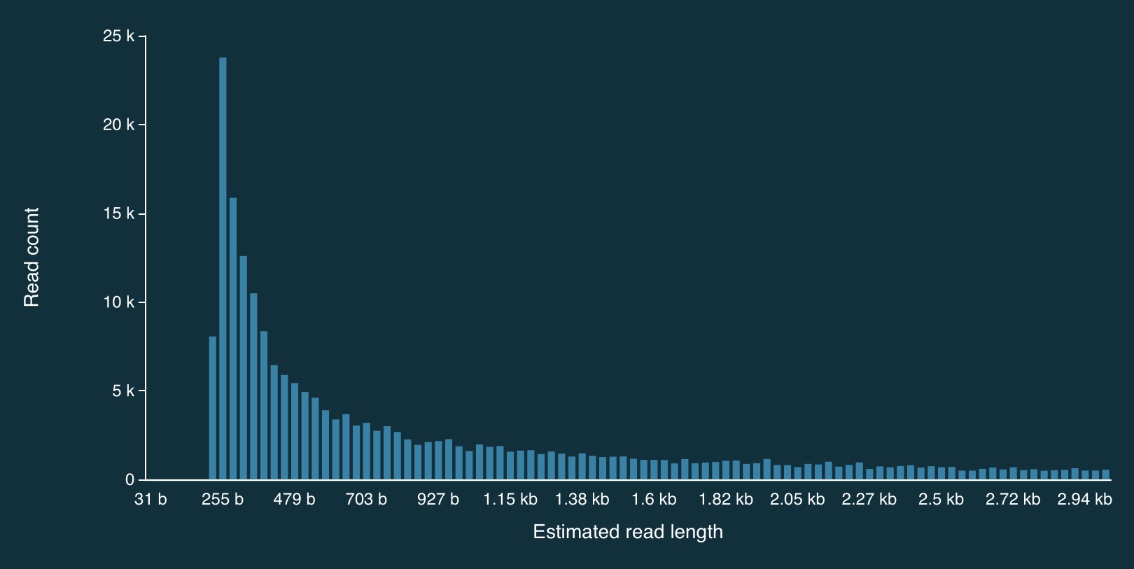
Distribution of read lengths
Here is the full distribution of read lengths without adaptive sampling turned on (i.e., I also ran a simulation without adaptive sampling) - there are LOTS of reads that less than 1000bp long:
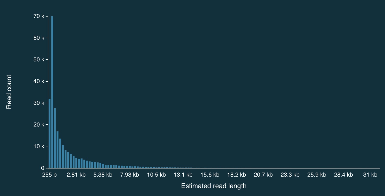
Here is a zoomed in view:
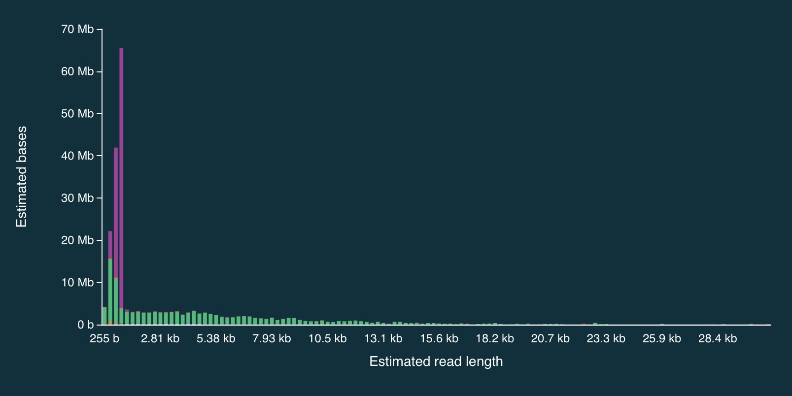
Adaptive sampling results
Despite the caveats, it is fairly clear that the adaptive sampling algorithm worked (or at least that it did something). In the plots below, the green bars represent reads that were not unblocked (i.e., the AS algorithm either: (1) decided the read mapped to a region in our bed file and continued sequencing it until the end, or (2) completed sequenced before a decision had been made), while the purple bars represent reads that were unblocked (i.e., the read was mapped in real-time, and the AS algorithm decided that it did not come from a region in our bed file, so ejected the read from the pore).
Here is the full distribution:
And here is a close up:
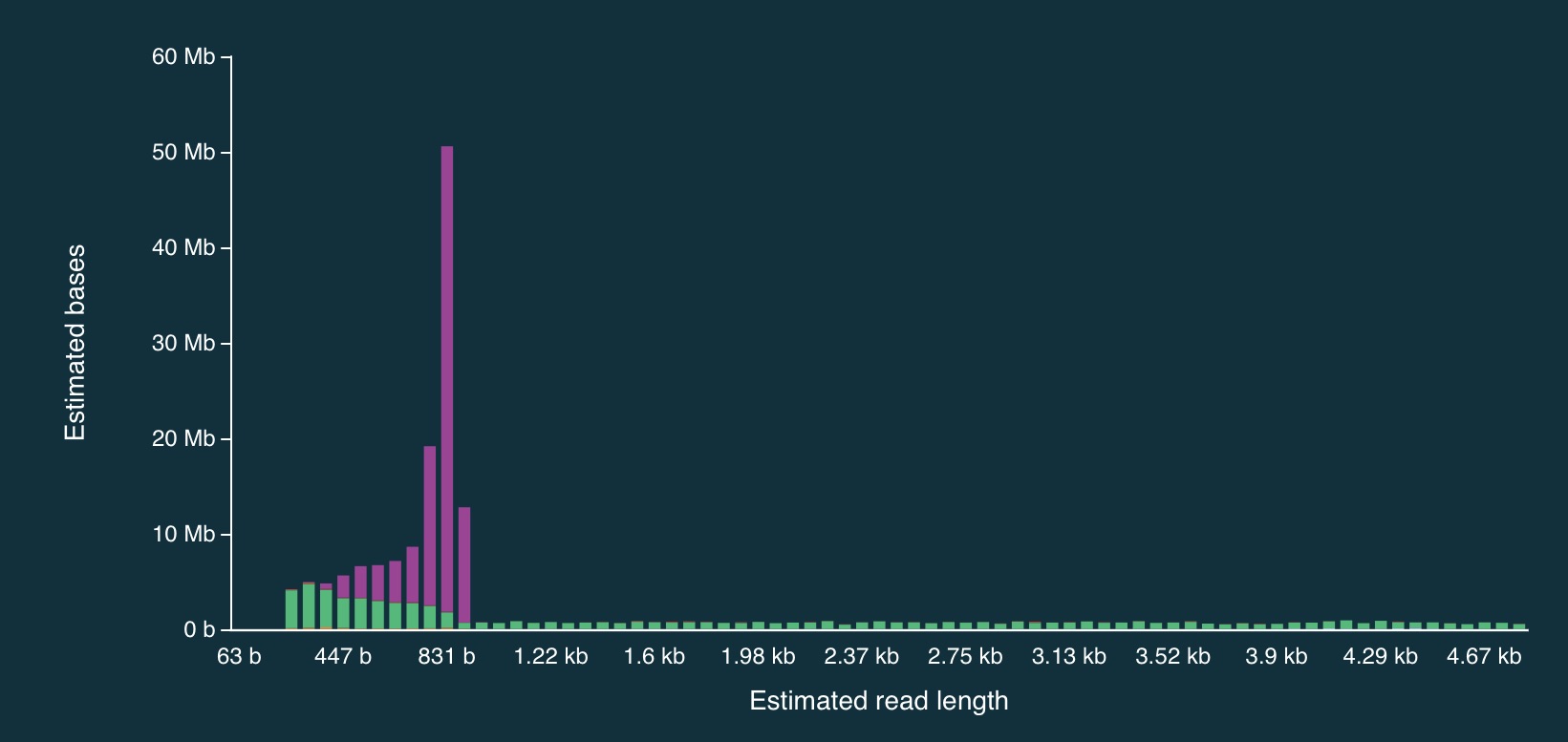
It is clear from the plots that the length of reads receiving an “unblock” signal is around 800bp, reflecting the time that the AS algorithm takes to make a decision about whether or not to reject a read.
Adaptive sampling details
NOTE: the information below may now be out of date…
When adaptive sampling is enabled, an additional output file is created, providing information about every read that was processed.
It is stored in the other_reports folder within the run directory, and is in CSV format. The naming convention is:
adaptive_sampling_XXX_YYY.csv
where XXC and YYY are flowcell and run identifiers (I think).
The format is:
batch_time,read_number,channel,num_samples,read_id,sequence_length,decision
1669157044.6601431,499,3,4008,bc65b9b4-bc05-45c4-a7b3-4c199577c8c9,350,unblock
1669157045.2247138,301,131,4000,1892041e-71a5-4121-9547-49122e247172,258,unblock
1669157045.2247138,438,42,4002,6be52363-5315-445c-bcd4-3d3b32a829dc,312,stop_receiving
1669157045.2247138,590,76,4001,e459305c-288d-47e7-9bbd-93224ee45074,264,unblock
1669157045.2247138,280,95,4005,a15f9aef-9b60-4f8f-bb74-c96b6f4fa16f,360,stop_receiving
1669157045.2247138,598,94,4001,8f615191-d1d4-42c5-a778-92c91411979b,357,unblock
1669157045.2247138,554,125,4003,8e628f9d-ae37-499e-b32e-7842bcf1539f,364,stop_receiving
1669157045.2247138,431,110,4003,12516158-8ed0-4bf2-bdff-f94171593996,378,unblock
1669157045.2247138,414,102,4008,1cad751a-ddde-4700-bb06-9dcf8974185a,313,unblock
Or slightly nicer (commas exchanged for tabs):
batch_time      read_number     channel num_samples          read_id        sequence_length     decision
1669157044.6601431      499     3       4008    bc65b9b4-bc05-45c4-a7b3-4c199577c8c9    350     unblock
1669157045.2247138      301     131     4000    1892041e-71a5-4121-9547-49122e247172    258     unblock
1669157045.2247138      438     42      4002    6be52363-5315-445c-bcd4-3d3b32a829dc    312     stop_receiving
1669157045.2247138      590     76      4001    e459305c-288d-47e7-9bbd-93224ee45074    264     unblock
1669157045.2247138      280     95      4005    a15f9aef-9b60-4f8f-bb74-c96b6f4fa16f    360     stop_receiving
1669157045.2247138      598     94      4001    8f615191-d1d4-42c5-a778-92c91411979b    357     unblock
1669157045.2247138      554     125     4003    8e628f9d-ae37-499e-b32e-7842bcf1539f    364     stop_receiving
1669157045.2247138      431     110     4003    12516158-8ed0-4bf2-bdff-f94171593996    378     unblock
1669157045.2247138      414     102     4008    1cad751a-ddde-4700-bb06-9dcf8974185a    313     unblock
Processing adaptive sampling data
Once the data have been generated, they are processed in exactly the same way:
- Basecalling with
dorado - QA/QC with FastQC and/or NanoPlot
- Alignment with
minimap2(viadorado)
I’ve done the above, and a bam file (wih an annoyingly long name) can be found at:
bam-files/yog-as-100kb-chunks-bed-SUP-pass-aligned-sort.bam
There are also a few additional things we can do to check how well the adaptive sampling has worked.
Filtering for read length
Because there are so many short reads (i.e., < 1000 bases) it is actually quite difficult to see the effect of adaptive sampling in this data set. To overcome this, we can remove these short reads from the data.
To do this, we can use SAMtools to filter the bam file.
First, load the SAMtools module:
module load SAMtools
Then filter:
samtools view -h bam-files/yog-as-100kb-chunks-bed-SUP-pass-aligned-sort.bam | \
   awk 'length($10) > 1000 || $1 ~ /^@/' | \
   samtools view -bS - > bam-files/yog-as-100kb-chunks-bed-SUP-pass-aligned-sort-LONG-1KB.bam
And then index the new file:
samtools index bam-files/yog-as-100kb-chunks-bed-SUP-pass-aligned-sort-LONG-1KB.bam
Now we have a new bam file that only contains aligned reads longer than 1000bp.
Checking the read depth of the selected regions
We can use samtools bedcov to calculate how much sequence data was generated for specific regions of the genome.
For this, we need a bed file. This one breaks the 1.8Mbp S. thermophilus genome into 100Kbp chunks (admitedly, I missed a little bit of the end - after 1,800,000bp):
NZ_LS974444.1   0       99999
NZ_LS974444.1   100000  199999
NZ_LS974444.1   200000  299999
NZ_LS974444.1   300000  399999
NZ_LS974444.1   400000  499999
NZ_LS974444.1   500000  599999
NZ_LS974444.1   600000  699999
NZ_LS974444.1   700000  799999
NZ_LS974444.1   800000  899999
NZ_LS974444.1   900000  999999
NZ_LS974444.1   1000000 1099999
NZ_LS974444.1   1100000 1199999
NZ_LS974444.1   1200000 1299999
NZ_LS974444.1   1300000 1399999
NZ_LS974444.1   1400000 1499999
NZ_LS974444.1   1500000 1599999
NZ_LS974444.1   1600000 1699999
NZ_LS974444.1   1700000 1799999
Aside: how can we generate a file like that?
Let’s build one with bash!
First, let’s write a loop that counts from 1 to 10 in steps of 2:
for i in {1..10..2}
do
    echo $i
done
1
3
5
7
9
Now lets do 0 to 1,799,999, in steps of 100,000:
for i in {0..1799999..100000}
do
    echo $i
done
0
100000
200000
300000
400000
500000
600000
700000
800000
900000
1000000
1100000
1200000
1300000
1400000
1500000
1600000
1700000
Add the chromosome name, and the end position to each line (and make sure to separate with tabs):
for i in {0..1799999..100000}
do
    start=$i
    end=`echo $i+99999 | bc`
    echo -e NZ_LS974444.1'\t'$start'\t'$end
done
NZ_LS974444.1   0       99999
NZ_LS974444.1   100000  199999
NZ_LS974444.1   200000  299999
NZ_LS974444.1   300000  399999
NZ_LS974444.1   400000  499999
NZ_LS974444.1   500000  599999
NZ_LS974444.1   600000  699999
NZ_LS974444.1   700000  799999
NZ_LS974444.1   800000  899999
NZ_LS974444.1   900000  999999
NZ_LS974444.1   1000000 1099999
NZ_LS974444.1   1100000 1199999
NZ_LS974444.1   1200000 1299999
NZ_LS974444.1   1300000 1399999
NZ_LS974444.1   1400000 1499999
NZ_LS974444.1   1500000 1599999
NZ_LS974444.1   1600000 1699999
NZ_LS974444.1   1700000 1799999
Using samtools bedcov
Once we’ve got a bed file, samtools bedcov can be used to calculate the amount of sequence generated for the
regions in the bed file.
I’ve generated a longer bed file, splitting the genome into 10Kb chunks. It can be found at:
bed-files/chunks-10k.bed
Now let’s use this file with samtools bedcov:
samtools bedcov bed-files/chunks-10k.bed \
   bam-files/yog-as-100kb-chunks-bed-SUP-pass-aligned-sort-LONG-1KB.bam
First 20 rows:
NZ_LS974444.1   0       9999    1971063
NZ_LS974444.1   10000   19999   1311458
NZ_LS974444.1   20000   29999   1276564
NZ_LS974444.1   30000   39999   1744496
NZ_LS974444.1   40000   49999   1665578
NZ_LS974444.1   50000   59999   420445
NZ_LS974444.1   60000   69999   350856
NZ_LS974444.1   70000   79999   1138767
NZ_LS974444.1   80000   89999   1320115
NZ_LS974444.1   90000   99999   1393254
NZ_LS974444.1   100000  109999  415558
NZ_LS974444.1   110000  119999  131388
NZ_LS974444.1   120000  129999  189621
NZ_LS974444.1   130000  139999  156248
NZ_LS974444.1   140000  149999  154235
NZ_LS974444.1   150000  159999  127957
NZ_LS974444.1   160000  169999  105826
NZ_LS974444.1   170000  179999  105900
NZ_LS974444.1   180000  189999  61800
NZ_LS974444.1   190000  199999  315476
Write it to a text file:
mkdir coverage-files
samtools bedcov bed-files/chunks-10k.bed \
   bam-files/yog-as-100kb-chunks-bed-SUP-pass-aligned-sort-LONG-1KB.bam > \
   coverage-files/yog-as-100kb-chunks-10k-cov.txt
We’ll use this to make a plot of read depth across the genome in R.
But first…
Another aside: complementing a bed file
If you have a bed file containing genomic regions that have been used for adaptive sampling, it can be useful to create a second bed file that containing the complement of these regions (i.e., the regions of the genome that were not being selected via adaptive sampling). This can be used to check read depth at non-selected regions.
To do this, we first index the reference genome using samtools:
samtools faidx genome/streptococcus-thermophilus-strain-N4L.fa
This produces the file: streptococcus-thermophilus-strain-N4L.fa.fai:
more genome/streptococcus-thermophilus-strain-N4L.fa.fai
NZ_LS974444.1 1831756 66 70 71
We can use this to extract chromosome sizes (in this case, there is only one, but for multi-chromosome genomes - e.g., human - this is a really useful approach):
cut -f 1,2 genome/streptococcus-thermophilus-strain-N4L.fa.fai > genome/st-chrom-sizes.txt
The cut command splits lines of text into separate “fields” - by default, “tab” is used as the delimiter (others can be specified).
In this case, the code just takes the first two fields, which are the chromosome name and length.
Check what it produced:
more genome/st-chrom-sizes.txt
NZ_LS974444.1 1831756
This information can then be used to create the complement bed file:
module load BEDTools
bedtools complement -i bed-files/as-100kb-chunks.bed -g genome/st-chrom-sizes.txt > bed-files/as-100kb-chunks-complement.bed
more bed-files/as-100kb-chunks-complement.bed
NZ_LS974444.1   99999   200000
NZ_LS974444.1   299999  400000
NZ_LS974444.1   499999  600000
NZ_LS974444.1   699999  800000
NZ_LS974444.1   899999  1000000
NZ_LS974444.1   1099999 1200000
NZ_LS974444.1   1299999 1400000
NZ_LS974444.1   1499999 1600000
NZ_LS974444.1   1699999 1831756
Check (visually) that this is the complement of the bed file I used for adaptive sampling:
more bed-files/as-100kb-chunks.bed
NZ_LS974444.1   0       99999
NZ_LS974444.1   200000  299999
NZ_LS974444.1   400000  499999
NZ_LS974444.1   600000  699999
NZ_LS974444.1   800000  899999
NZ_LS974444.1   1000000 1099999
NZ_LS974444.1   1200000 1299999
NZ_LS974444.1   1400000 1499999
NZ_LS974444.1   1600000 1699999
We can use these files with samtools bedcov to generate read depth information separately for the
selected and non-selected regions (handy if you AS selection is somewhat complex - e.g., all exons, a specific set of genes etc).
Coverage info for selected regions:
samtools bedcov bed-files/as-100kb-chunks.bed \
   bam-files/yog-as-100kb-chunks-bed-SUP-pass-aligned-sort-LONG-1KB.bam > \
   coverage-files/yog-as-100kb-chunks-SELECTED-cov.txt
Coverage info for non-selected regions:
samtools bedcov bed-files/as-100kb-chunks-complement.bed \
   bam-files/yog-as-100kb-chunks-bed-SUP-pass-aligned-sort-LONG-1KB.bam > \
   coverage-files/yog-as-100kb-chunks-NONSELECTED-cov.txt
more coverage-files/yog-as-100kb-chunks-SELECTED-cov.txt
NZ_LS974444.1   0       99999   12593594
NZ_LS974444.1   200000  299999  14610340
NZ_LS974444.1   400000  499999  12060688
NZ_LS974444.1   600000  699999  14714058
NZ_LS974444.1   800000  899999  16128475
NZ_LS974444.1   1000000 1099999 15793991
NZ_LS974444.1   1200000 1299999 17615309
NZ_LS974444.1   1400000 1499999 13341368
NZ_LS974444.1   1600000 1699999 16061631
more coverage-files/yog-as-100kb-chunks-NONSELECTED-cov.txt
NZ_LS974444.1   99999   200000  1764394
NZ_LS974444.1   299999  400000  1738930
NZ_LS974444.1   499999  600000  1736471
NZ_LS974444.1   699999  800000  1602761
NZ_LS974444.1   899999  1000000 1739915
NZ_LS974444.1   1099999 1200000 2134827
NZ_LS974444.1   1299999 1400000 4654002
NZ_LS974444.1   1499999 1600000 3945477
NZ_LS974444.1   1699999 1831756 2277969
Some quick analysis in R
Choose “New Launcher” from the file menu, and start an RStudio session.
In R, you might need to set your working directory to be the adaptive-sampling directory:
setwd('~/obss_2023/nanopore/adaptive-sampling/')
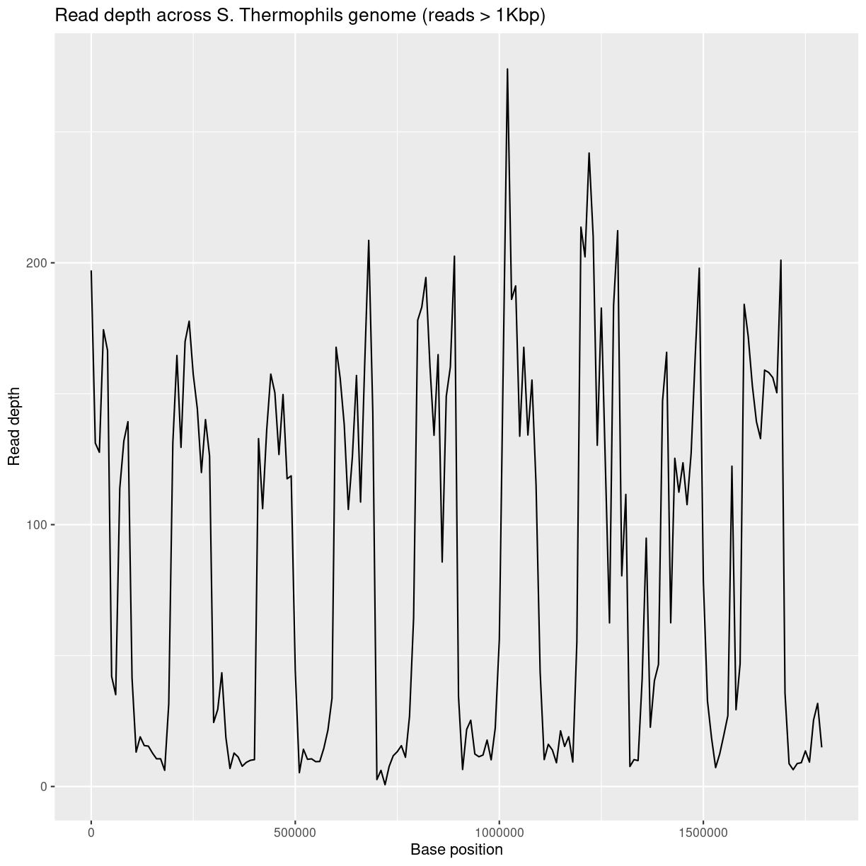
Genome-wide read-depth
Load the dplyr and ggplot2 packages:
library(ggplot2)
library(dplyr)
Load the text file that we generated using samtools bedcov:
bedCov = read.table('coverage-files/yog-as-100kb-chunks-10k-cov.txt', header=FALSE, sep='\t')
Take a look at the data:
head(bedCov)
             V1    V2    V3      V4
1 NZ_LS974444.1     0  9999 1971063
2 NZ_LS974444.1 10000 19999 1311458
3 NZ_LS974444.1 20000 29999 1276564
4 NZ_LS974444.1 30000 39999 1744496
5 NZ_LS974444.1 40000 49999 1665578
6 NZ_LS974444.1 50000 59999  420445
Add some column names:
names(bedCov) = c("CHROM", "START", "END", "BASES")
Add columns for region length (LENGTH) and then calculated average read depth (DEPTH):
bedCov = mutate(bedCov, LENGTH = END - START + 1)
bedCov = mutate(bedCov, DEPTH = BASES / LENGTH)

head(bedCov)
          CHROM START   END   BASES LENGTH    DEPTH
1 NZ_LS974444.1     0  9999 1971063  10000 197.1063
2 NZ_LS974444.1 10000 19999 1311458  10000 131.1458
3 NZ_LS974444.1 20000 29999 1276564  10000 127.6564
4 NZ_LS974444.1 30000 39999 1744496  10000 174.4496
5 NZ_LS974444.1 40000 49999 1665578  10000 166.5578
6 NZ_LS974444.1 50000 59999  420445  10000  42.0445
ggplot(bedCov, aes(x=START, y=DEPTH)) +
  geom_line() +
  ggtitle("Read depth across S. Thermophils genome (reads > 1Kbp)") +
  xlab("Base position") + ylab("Read depth")
Average read-depth in selected and non-selected regions
bedCovSelected = read.table('coverage-files/yog-as-100kb-chunks-SELECTED-cov.txt', header=FALSE, sep='\t')
names(bedCovSelected) = c("CHROM", "START", "END", "BASES")
bedCovSelected = mutate(bedCovSelected, LENGTH = END - START + 1)
bedCovSelected = mutate(bedCovSelected, DEPTH = BASES / LENGTH)
Calculate average read depth for selected regions:
mean(bedCovSelected$DEPTH)
[1] 147.6883
Exercise: calculating read-depth
- Repeat the average read depth calculation for the non-selected regions.
- Was the average read depth different between the two regions?
Solution
bedCovNonSelected = read.table('coverage-files/yog-as-100kb-chunks-NONSELECTED-cov.txt', header=FALSE, sep='\t')

names(bedCovNonSelected) = c("CHROM", "START", "END", "BASES")

bedCovNonSelected = mutate(bedCovNonSelected, LENGTH = END - START + 1)
bedCovNonSelected = mutate(bedCovNonSelected, DEPTH = BASES / LENGTH)

mean(bedCovNonSelected$DEPTH)
Average read depth for non-selected regions is: 23.38
This is A LOT less than the average read depth for the selected regions: 147.69
Key Points
Nanopore can determine if it should continue to sequence a read.