library(tidyverse)
library(palmerpenguins)

# brings 'penguins' dataset into name space
attach(penguins)
# brings 'penguins_raw' dataset into name space
attach(penguins_raw)
Multi-plots
Setup
Multi-plots with Patchwork
The {patchwork} package is great for assembling multiple plots into a single plot
Documentation for {patchwork}: https://patchwork.data-imaginist.com/index.html
library(patchwork)Lets create some example plots that we can call upon
penguin_point_plot <- ggplot(
  data = penguins,
  mapping = aes(x = body_mass_g,
                y = flipper_length_mm,
                colour = island)
) +
  geom_point() +
  ggtitle("Plot 1")


penguin_box_plot <- ggplot(
  data = penguins,
  mapping = aes(x = species,
                y = flipper_length_mm)
) +
  geom_boxplot() +
  ggtitle("Plot2")
Different ways of combining plots
side by side using +
penguin_point_plot + penguin_box_plotWarning: Removed 2 rows containing missing values or values outside the scale range
(`geom_point()`).Warning: Removed 2 rows containing non-finite outside the scale range
(`stat_boxplot()`).
Or use | to create columns in the layout
penguin_point_plot | penguin_box_plotWarning: Removed 2 rows containing missing values or values outside the scale range
(`geom_point()`).Warning: Removed 2 rows containing non-finite outside the scale range
(`stat_boxplot()`).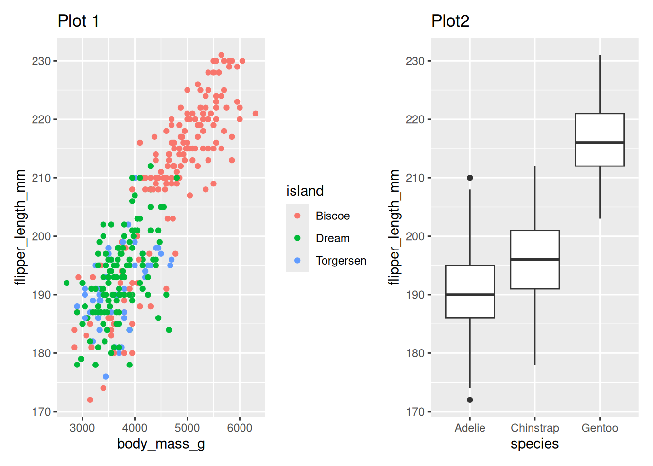
One over the other using /
penguin_point_plot / penguin_box_plotWarning: Removed 2 rows containing missing values or values outside the scale range
(`geom_point()`).Warning: Removed 2 rows containing non-finite outside the scale range
(`stat_boxplot()`).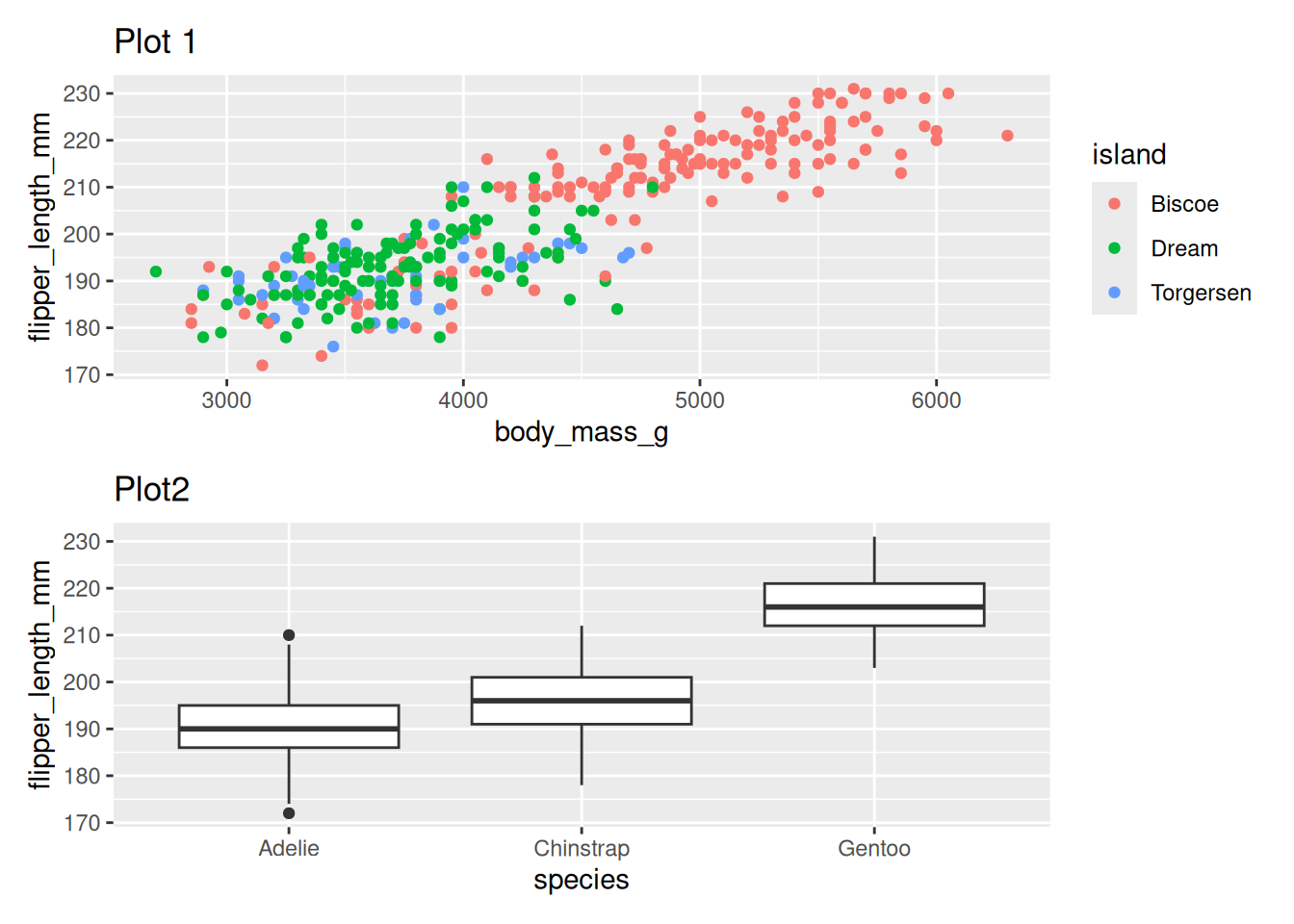
Including a table
library(gt)
penguin_tab <- penguins %>%
  group_by(species) %>%
  summarise(n = n()) %>%
  gt()
penguin_point_plot + penguin_tabWarning: Removed 2 rows containing missing values or values outside the scale range
(`geom_point()`).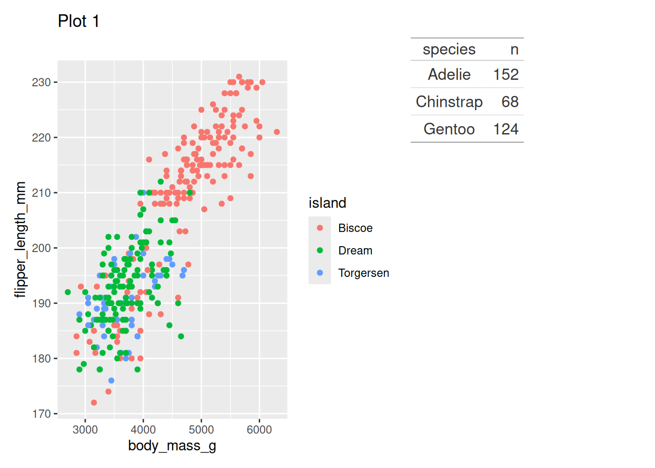
Controlling Layouts with plot_layout()
The {patchwork} package has the ability to control layouts through several methods (rows/columns, relative sizes, and custom designs). Below are short examples using the plots and table defined earlier.
- Use plot_layout() to set number of columns and relative widths/heights.
- Use parentheses to group stacked/side-by-side operators when you want to apply layout options to the combined result.
- Use a design string to create more complex placements (one plot spanning multiple cells).
- Collect legends with guides = “collect” and add a shared title with plot_annotation().
# example plots
p1 <- ggplot(penguins, aes(x = body_mass_g, y = flipper_length_mm, colour = species)) +
  geom_point(na.rm = TRUE) + ggtitle("Mass vs Flipper")

p2 <- ggplot(penguins, aes(x = species, y = flipper_length_mm)) +
  geom_boxplot(na.rm = TRUE) + ggtitle("Flipper by species")

p3 <- ggplot(penguins, aes(x = island, y = body_mass_g)) +
geom_violin(na.rm = TRUE) + ggtitle("Mass by island")- An example two-column layout where p1 takes left column and p2/p3 stack on the right
widthsis specifying the width of each column
(p1 | (p2 / p3)) +
  plot_layout(widths = c(2, 1)) +
  plot_annotation(title = "p1 large left, p2 & p3 stacked right")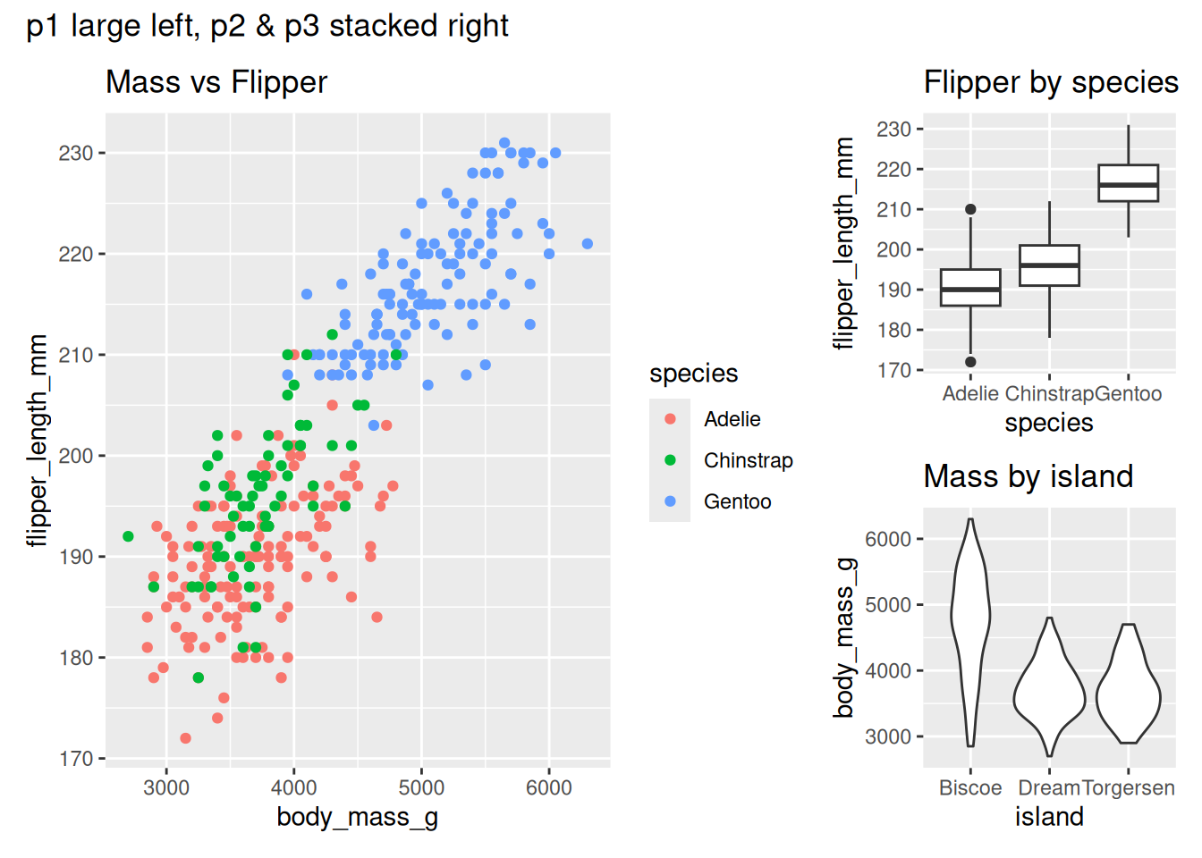
- Grid layout with relative widths/heights and a shared legend collected
(p1 + p2 + p3) +
  plot_layout(ncol = 2, widths = c(2, 1), heights = c(1, 1), guides = "collect") + #&
  # theme(legend.position = "bottom") +
  plot_annotation(tag_levels = "A")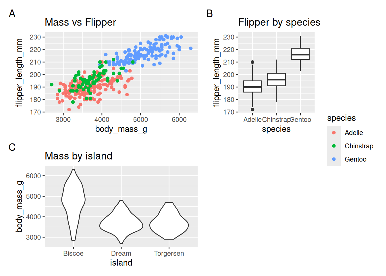
- Complex placement using a design string (A spans 3 cells in row 1)
#is used as a ‘spacer’ or empty plot
design <- "
AAA
B#C
"
p1 + p2 + p3 + plot_layout(design = design) +
  plot_annotation(title = "Design string layout")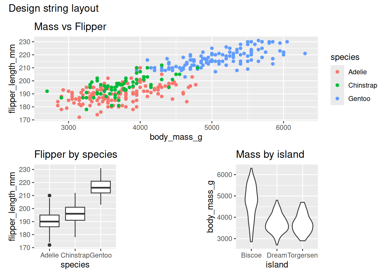
Alternatively, plot_spacer() can be used in the plot specification and it’s treated as a plot within the design (instead of using “#”).
design <- "
AAA
BCD
"
p1 + p2 + plot_spacer() + p3 + plot_layout(design = design) +
  plot_annotation(title = "Design string layout")
Notes: use widths/heights for relative sizing, guides = “collect” to share legends, and a design string for precise cell placement.