coldata <- read.table("https://raw.githubusercontent.com/GenomicsAotearoa/RNA-seq-data-analysis-workflow-NZ/refs/heads/main/data-files/coldata.txt", sep="\t", header=TRUE)
counts <- read.table("https://raw.githubusercontent.com/GenomicsAotearoa/RNA-seq-data-analysis-workflow-NZ/refs/heads/main/data-files/counts.txt", sep="\t", header=TRUE, row.names=1)Identify Differentially Expressed Genes
Statistical approach
In order to identify which genes are differentially expressed between two groups (in this case, we have 15 samples from three phenotypes), when need to test if groups are significantly different from one another, which can be a challenging question to answer. We can start by specifically asking our question as a statistical question: Are the differences we observe between two groups greater than the differences we would expect to see by chance?
In the interest of time, in this workshop we will not get into T-tests, P-values and types of errors. You can read more about that here:
Statistics 📊
T-tests and p-values
The statistical approach to this question is to begin with the null hypothesis (that there is no difference between the two groups) and test whether or not you can reject the null hypothesis.
To test whether or not we can reject the null hypothesis we can calculate a test statistic:
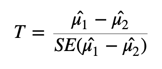
Here we are taking the difference between the means of the two groups and then dividing that difference by some measure of variability - in this case, dividing by the standard error.
If the difference in means is LARGE relative to the variance, the test statistic will be large (indicating significance). If the difference between the means is small relative to the variance, the test statistic will be small, indicating the difference is probably not significant (i.e., the difference we observe is in-line with the variance we observe).
🧠🏋️♀️ EXERCISE (1 min)
With the above formula in mind, what impact would heteroscedasticity have when you are attempting to identify differentially expressed genes?
SOLUTION
Heteroscedasticity would violate the assumption of equal variances that the t-statistic relies on, meaning the standard error \({SE(\hat{\mu}_1 - \hat{\mu}_2)}\) no longer appropriately captures the variability between groups. This would produce unreliable test statistics and therefore untrustworthy p-values. Therefore you could no longer confidently determine whether an observed difference in gene expression between groups was real or due to chance.
Interpreting p-values
Once we have a test statistic we will calculate a p-value. The p-value is an indication of how likely we were to observe the given difference in means (or a more extreme difference) if there is truly no difference between the means. That is, how likely are we to see this difference due to random chance?
How do we interpret the p-value? We will specify a threshold (usually 0.05), and say that if a p-value is less than this threshold we will consider it a significant result. If the p-value is lower than the threshold we set, we will reject the null hypothesis (that the groups are identical) and accept the alternative (that there is a difference between the groups). The threshold we set is our level of “risk” that this event happened by chance alone.
When we declare that a result with a p-value of less than 0.05 is significant, we are saying that we believe the difference to be true since, if there was truly no difference, such a result would happen less than 5% of the time.
A useful mental analogy is to consider flipping a coin. We know that for a fair coin, the odds of getting heads is 50:50. Still, if we get four heads in a row it doesn’t worry us - it’s entirely plausible given the variation we expect. But if we get 50 heads in a row, while we know it’s statistically possible, we know it’s very unlikely to see such an extreme result. If we got to 100 heads in a row, we might instead start to question the fairness of the coin - we would reject the null hypothesis that the odds of heads and tails is identical.
Types of errors
It’s important to think about the two possible ways in which we could be wrong when testing a hypothesis like this: we could generate a false positive or a false negative.
A false positive or Type I error is when we reject the null hypothesis when there is truly no significant difference.
A false negative or Type II error is when we fail to reject the null hypothesis when there truly is a significant difference.
When we select a p-value threshold of 0.05, we are accepting the fact that 5% of the time that the null hypothesis is true, we will reject it. This becomes hugely problematic when you are testing thousands of genes! In order to avoid a large number of false positives we must correct for multiple testing. The more tests we are doing, the more stringent we need to be. We will not cover multiple testing corrections in depth but will briefly mention two types:
Family-wise Error Rate (FWER), also called the Bonferroni and Holm corrections, is a highly stringent procedure. This approach will give the minimal possible number of false positives, but will miss some true positives. Good if false positives are particularly costly (e.g., if you are providing someone with a severe medical diagnosis).
False Discovery Rate control (FDR), also called the Benjamini and Hochberg correction, is less conservative than FWER. This approach will identify more significant events, but expect a greater number of false positives. Use this approach if you are more concerned about missing something valuable and can afford a few false positives.
🧠🏋️♀️ EXERCISE (3 mins)
Note down some key features of your experiment. Are you more inclined to use FWER or FDR? Which is more appropriate for your data and your experimental situation?
Food for thought
- Are you working with clinical samples, where the stakes are higher if you implicate the wrong gene in disease?
- Are you investigating trends in expression or looking for specific genes?
- How radical is your treatment or conditions used in your experiment? Do you have any assumptions about how perturbed or different you expect gene expression to be between sample groups?
- How many biological replicates do you have? Smaller sample sizes reduce statistical power, making you more prone to Type II errors regardless of which correction you apply.
Modifying the t-test and variance shrinkage for RNA-seq
Many biological experiments struggle with getting enough samples for statistical significance. In RNA-seq experiments it is common to see groups of three samples or replicates. This is especially problematic when using the t-test (or similar procedures that involve variance). When testing for differences in gene expression it is possible to encounter genes with a small difference in the mean between the two groups and, due to the small sample size, a very small level of variation (a small standard error). A small difference in the means divided by a very small standard error translates to a large test statistic, which is then translated to a small p-value and what looks like a highly significant result.
Since this issue is caused by an artificially low standard error (unreliable variance estimates) due to low sample numbers, a number of methods stabilise the standard error in some way. One way to implement this is through shrinkage estimation, which involves using Empirical Bayes methods to adjust the variance estimates of individual genes based on the overall distribution of variances. During shrinkage estimation, small variances are made larger while large variances are made smaller. Limma applies this directly to the variance in a moderated t-test. DESeq2 models counts with a negative binomial distribution and instead shrinks the gene-wise dispersion toward a mean-dependent trend, then tests with GLM (generalised linear model) based tests.
In summary:
- The “standard” P-value cut-off of 0.05 is not sufficient – 5% results in too many genes that will be false positives (i.e., genes that look like they are DE, but they are not).
- We need to use a p-value correction - usually FDR, also called Benjamini and Hochberg correction, but if you want to be more strict use FWER.
- We must correct for heteroscedasticity, i.e., variance is dependent on the mean.
Identifying differentially expressed genes using DESeq2
DESeq2 is a highly-regarded R package for analysing RNA-seq data. DESeq2 uses a negative binomial method to model the count data, and combines this with a generalised linear model (GLM) to identify differentially expressed genes. For more about the DESeq2 package, you can read the original article.
Need to load in the data again?
Run this code to load in the data:
The DESeq2 object
The DESeq2 package requires a specific data storage object called a “DESeq Data Set” or DDS object. The DDS object contains not just the count data, but also the metadata and the design matrix. This object can be created using a function from the DESeq2 package called DESeqDataSetFromMatrix() Once we have created the dds object, we can view the data stored within using the counts function.
Important! Check sample names are in the same order for both objects
First make sure the sample names in coldata and counts match each other and are in the same order. If they don’t match or are not in the same order, the dge object and design matrix won’t match and the result will be the wrong metadata being attributed to the wrong sample.
Run this code to force the coldata sample column match the same order as the coldata column names. Check that they are identical (should return TRUE, then you are good to continue if so). If not, check your coldata and counts objects to see what is different.
coldata <- coldata[match(colnames(counts), coldata$sample), ] # force columns into same sample order
identical(colnames(counts), coldata$sample) # must be TRUE
[1] TRUElibrary(tidyverse)
library(DESeq2)
coldata$histology <- factor(coldata$histology, levels = c("F", "MT", "TPM"))
coldata$batchname <- factor(coldata$batchname)
dds <- DESeqDataSetFromMatrix(countData = counts,
colData = coldata,
design = ~histology + batchname)
Why factorise?
This is not strictly necessary – the code won’t break, as DESeq2 will automatically convert character columns to factors (although numeric columns will likely error and must be factorised first!)
But in our case we want to set an order, which we should do with factor().
This is because F, MT, and TPM represent a chronological transition in state (i.e., gonads transition from female –> multiple distinct transitional states –> terminal phase male), and we want this order reflected in our results. The same order also comes up when using ggplot2, if we want the x-axis to plot in a specific order rather than alphabetically.
The design matrix can be pulled directly from the data provided to the colData argument.
Alternatively, use design = ~1 to fit an intercept-only model (no condition effect), useful for testing out normalisation or transformation steps where group comparisons aren’t needed.
Raw counts can be retrieved from our dds object using the function counts() from the DESeq2 package.
counts(dds) |> head() SI16_21G SI16_23G SI18_30G SI18_48G SI18_52G SI16_22G SI18_15G
LOC117820358 0 0 0 0 0 0 0
LOC117813751 0 0 0 0 0 5 0
ccdc51 55 62 63 46 93 57 83
tma7 1256 2246 1492 1870 1664 2506 1514
LOC117815572 2 1 2 1 1 11 1
LOC117818779 0 1 0 0 0 2 2
SI18_16G SI18_18G SI18_22G SI16_1G SI16_2G SI16_3G SI18_47G
LOC117820358 0 0 0 0 0 0 0
LOC117813751 0 0 0 723 346 482 140
ccdc51 52 61 85 241 181 175 190
tma7 1322 1053 1129 3262 3098 3050 2336
LOC117815572 3 0 4 3 3 22 30
LOC117818779 2 0 1 0 3 0 16
SI18_49G
LOC117820358 0
LOC117813751 33
ccdc51 103
tma7 2245
LOC117815572 15
LOC117818779 0Now fit the DESeq2 generalised linear model to the data.
dds <- DESeq(dds)estimating size factorsestimating dispersionsgene-wise dispersion estimatesmean-dispersion relationshipfinal dispersion estimatesfitting model and testingNote the outputs from running this function. What are these outputs?
Estimating size factors: assesses library size and calculates factors to adjust for differences between samples. This also adjusts for compositional differences (e.g., if gene X in sample 1 takes up a very large proportion of all available reads, other genes will have correspondingly fewer genes. If this effect is not uniform across samples, it can be corrected for during this stage).
Dispersion: adjusting for heteroscedasticity. DESeq2 makes use of variability estimates from not just one gene, but from all genes to make estimates about overall levels of variance. By bringing in (or “borrowing”) information from other genes, DESeq2 compensates for a small number of samples (which can lead to artificially small variance estimates otherwise).
Fitting model and testing: fitting the GLM and identifying differentially expressed genes.
We will create a new object to store the results in. We can access those results using either the head function or the summary function, which will give us slightly different information – both are valid and useful ways of familiarising yourself with the data.
res_F_vs_TPM <- results(dds, contrast = c("histology", "F", "TPM"))

res_F_vs_TPM |> head()
log2 fold change (MLE): histology F vs TPM
Wald test p-value: histology F vs TPM
DataFrame with 6 rows and 6 columns
baseMean log2FoldChange lfcSE stat pvalue
<numeric> <numeric> <numeric> <numeric> <numeric>
LOC117820358 0.00000 NA NA NA NA
LOC117813751 72.65818 -9.183293 0.967298 -9.493757 2.22854e-21
ccdc51 94.55083 -0.984036 0.375143 -2.623093 8.71355e-03
tma7 1891.60802 -0.134454 0.297961 -0.451246 6.51812e-01
LOC117815572 4.59230 -2.576477 0.906197 -2.843174 4.46666e-03
LOC117818779 1.37837 -2.735360 1.823510 -1.500052 1.33601e-01
padj
<numeric>
LOC117820358 NA
LOC117813751 4.26248e-20
ccdc51 1.53114e-02
tma7 6.99225e-01
LOC117815572 8.37165e-03
LOC117818779 1.77923e-01
Why use log2 for fold change?
For RNAseq data, we always use log2 fold change (log2FC) rather than log10 or natural log transformations. You may remember we used log2 to transform our raw counts too for plotting in the Exploratory Analysis section. This is because the log2 scale is easier to intuitively interpret up- and down-regulation. A log2FC of 1 means the gene is expressed twice as much in one condition compared to another, while a log2FC of -1 means it is expressed half as much.
To visualise this further, take this example:
| Count | log2(count) | log10(count) |
|---|---|---|
| 2 | 1 | 0.301 |
| 4 | 2 | 0.602 |
| 8 | 3 | 0.903 |
| 100 | 6.644 | 2 |
| 200 | 7.644 | 2.301 |
Each doubling in count is represented by an increase in 1 on the log2 scale, while on the log10 scale, each doubling is represented by an increase of only 0.3.
Note that log2FC is the difference in log2(count) between two conditions, rather than the log2 of a single count. This naturally extends to negative log2FC values too: for example, a log2FC of -2 means the gene is expressed a quarter as much in one condition compared to another.
| Comparison (count) | Fold change | log2FC | log10FC |
|---|---|---|---|
| 100 → 200 | 2× | 1 | 0.301 |
| 100 → 400 | 4× | 2 | 0.602 |
| 100 → 50 | 0.5× | −1 | −0.301 |
| 100 → 25 | 0.25× | −2 | −0.602 |
res_F_vs_TPM |> summary()
out of 25904 with nonzero total read count
adjusted p-value < 0.1
LFC > 0 (up)       : 5654, 22%
LFC < 0 (down)     : 10960, 42%
outliers [1]       : 131, 0.51%
low counts [2]     : 2000, 7.7%
(mean count < 0)
[1] see 'cooksCutoff' argument of ?results
[2] see 'independentFiltering' argument of ?results
Bonus: view coefficients and pull out by name
We can also pull out the native comparisons that are generated during analysis using:
resultsNames(dds)[1] "Intercept" "histology_MT_vs_F" "histology_TPM_vs_F"
[4] "batchname_SI18_vs_SI16"This lists every coefficient DESeq2 estimated directly when fitting the model. Because we set F as the reference level for histology, DESeq2 estimated each other level against F – so resultsNames() gives us histology_MT_vs_F and histology_TPM_vs_F, but not MT_vs_TPM
We can pull either of these straight out by name:
res_MT_vs_F <- results(dds, name = "histology_MT_vs_F" ) name and contrast will give you identical results whenever the comparison you want is against the reference level (here, F). name is just a shortcut that skips DESeq2 recomputing the contrast. For any comparison that isn’t against the reference level (e.g. MT vs TPM), you must use contrast instead, since that comparison/coefficient was never directly estimated.
Handy tip!
Want to save and output your full results now as a nice human readable table? Convert the res object to a dataframe, and then read out the table as a tsv file:
res_F_vs_TPM_df <- res_F_vs_TPM |> as.data.frame()

write.table(res_F_vs_TPM_df, file = "results/deseq2_F-vs-TPM-results.tsv", sep = "\t", quote = FALSE, row.names = TRUE, col.names = NA)The res object contains information for all genes tested. It is practical to create a new object that contains only the genes we consider differentially expressed based on the thresholds (p-value, logFC) and methods (e.g., multiple testing adjustment) that suit our situation.
We will remove any rows that have NAs in the results object, then pull out only those with an adjusted p-value less than 0.05. Because the contrast we generated here is contrast = c("histology", "F", "TPM")) this means that all genes with a positive logFC are upregulated in the first condition “F”. We want genes that are upregulated in the second condition “TPM”. To get these, we can simply grab all genes that are less than -1 logFC because anything downregulated in the first condition “F” is inherently upregulated in the second condition “TPM”.
res_F_vs_TPM <- res_F_vs_TPM |> na.omit()

# Get dimensions
res_F_vs_TPM   |> dim()
[1] 23773 6# Keep all rows in the res object if the adjusted p-value < 0.05 AND the log2 fold change is less than -1.
resPadjLogFC_F_vs_TPM <- res_F_vs_TPM[res_F_vs_TPM$padj <= 0.05 & res_F_vs_TPM$log2FoldChange < -1,]
# Get dimensions
resPadjLogFC_F_vs_TPM |> dim() [1] 9534 6EXERCISE 🧠🏋️♀️ (2 mins) - Identify method for multiple testing corrections
Bioinformatics can often be something of a “black box” - we execute a function by feeding in some data, and get new data as output. It’s very easy to fall into the trap of believing your data without asking all the necessary questions. For example, we’ve just used an adjusted p-value for our threshold for significance. Did you question which method was used to adjust for multiple testing? See if you can identify, using the help menu, which method was used here. Try and specify a different method for multiple testing corrections and note how this alters your output.
SOLUTION
The ?results help info will show the default p adjustment method is pAdjustMethod = "BH". Further reading will show that options for this come from ?p.adjust, which lists the following options:
"holm", "hochberg", "hommel", "bonferroni", "BH", "BY", "fdr", "none"
The default BH method is Benjamini & Hochberg (or the FDR method), which is described here in the R documentation.
Volcano plots
Volcano plots are a useful and commonly used method to visualise differentially expressed genes within your data set.
In the following code we will first produce the volcano plot itself, which shows the distribution of all genes according to p-value and log2 fold change.
Statistical significance is often not the only measure we will use to call genes differentially expressed. It is common to apply an additional threshold of gene expression needing to double or halve to be considered differentially expressed. On the log2FC scale, this is log2(2) (i.e., a value > 1 or < -1).
Genes will be coloured based on whether they are up (red) or down (blue) regulated.
This plot is an important “sanity check”. We can logically check that our significant genes (in red) are those with both a p-value < 0.05 and a log2 fold change greater than 1 (which is equivalent to a doubling or halving of gene expression). If we observe red marked dots in the center or bottom of the plot, we could recognise an error has occurred.
# Set up data
pval_threshold <- 0.05
fc_threshold   <- 1

plot_data <- as.data.frame(res_F_vs_TPM) |>
  tibble::rownames_to_column("ID") |>
  mutate(
    logFC      = log2FoldChange,
    negLogAdjPval = -log10(padj),
    category = case_when(
      padj <= pval_threshold & logFC >=  fc_threshold ~ "Upregulated",
      padj <= pval_threshold & logFC <= -fc_threshold ~ "Downregulated",
      padj <= pval_threshold                          ~ "Passes P-value cut-off",
      TRUE                                            ~ "Not significant"
    )
)library(ggplot2)
# Create plot
p <- ggplot(plot_data, aes(x = logFC, y = negLogAdjPval, colour = category, text = ID)) +
geom_point(alpha = 0.6, size = 1.5) +
scale_colour_manual(values = c(
"Upregulated" = "red",
"Downregulated" = "blue",
"Passes P-value cut-off" = "grey40",
"Not significant" = "grey80"
)) +
geom_vline(xintercept = c(-fc_threshold, fc_threshold), linetype = "dashed") +
geom_hline(yintercept = -log10(pval_threshold), linetype = "dashed") +
labs(
title = "Volcano Plot of Differential Gene Expression",
subtitle = paste("Thresholds: |log2FC| >=", fc_threshold,
"and adjusted p-value <=", pval_threshold),
x = "log2 Fold Change",
y = "-log10(adjusted p-value)",
colour = "Differential Expression"
) +
theme_minimal() +
theme(
plot.title = element_text(hjust = 0.5, size = 16),
plot.subtitle = element_text(hjust = 0.5, size = 12)
)
# display plot
p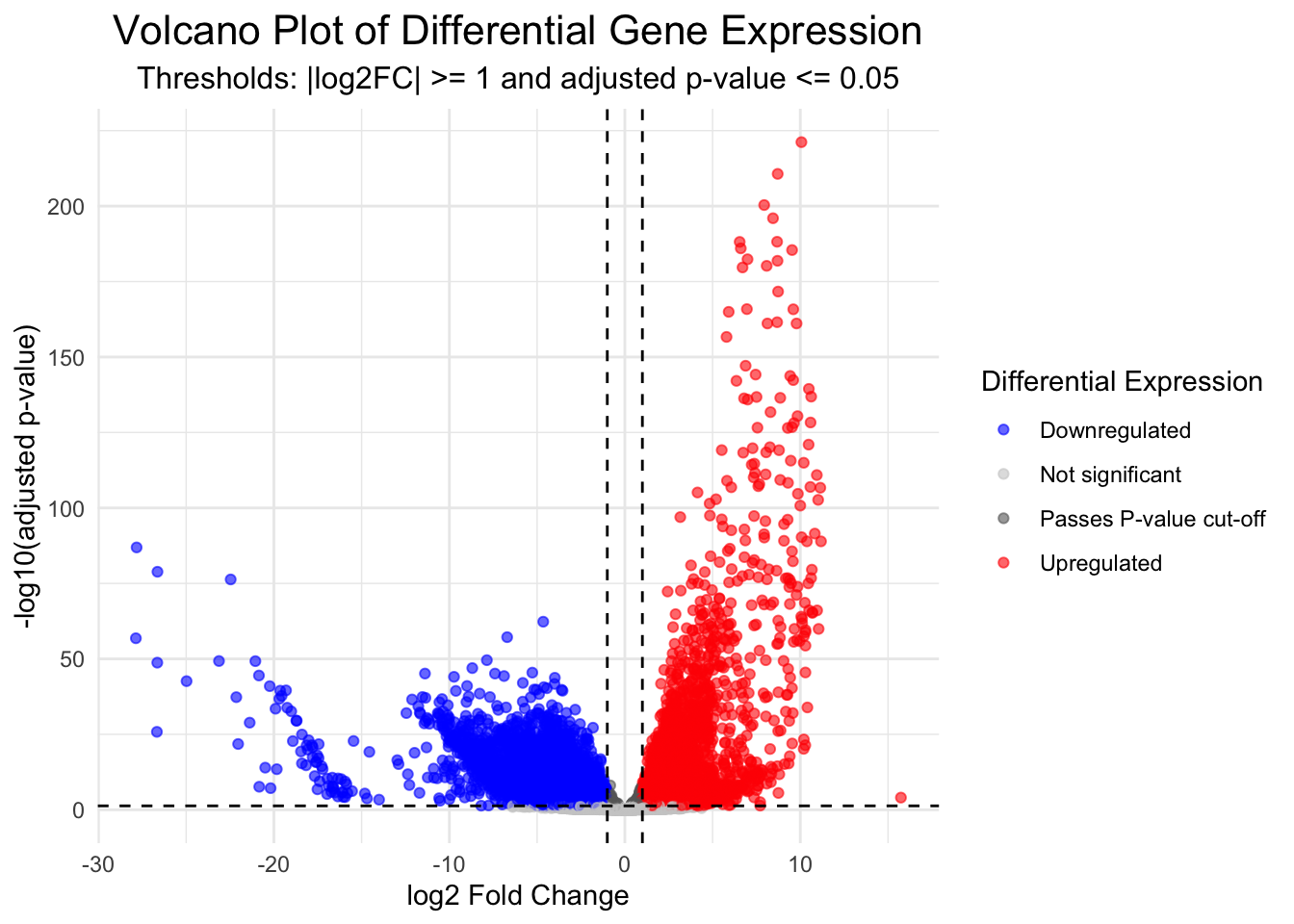
Convert to interactive volcano plot
library(ggiraph)
library(plotly)

# Convert ggplot to an interactive plotly object
interactive_plot <- ggplotly(p, tooltip = c("text", "x", "y", "colour"))

# Customise hover text
interactive_plot <- interactive_plot |>
  layout(hoverlabel = list(bgcolor = "white"),
         hovermode = "closest")

# Display the interactive plot
interactive_plot
# Save the plot (optional)
dir.create("plots")
ggsave("plots/volcano_plot_F_vs_TPM.png", width = 10, height = 8, dpi = 300)DISCUSSION 🤔 (2 mins)
We can see the blue dots are downregulated genes and the red dots are upregulated genes. But downregulated in what? Upregulated in what?
SOLUTION
It’s relative! The contrast we defined here was histology F vs TPM. Therefore, downregulated genes (blue) are those that are expressed less in TPM, than in F, while upregulated genes (red) are expressed more in TPM, than in F.
The opposite is also always true. Genes that are downregulated in TPM are upregulated in F, and vice versa. It’s always relative to the order in which we define the contrast and relative to the groups being compared.
Interactive Volcano plot
We can also produce an interactive volcano plot with the ggigraph package.
Hint: you should not need to change any of this code below to work with your data, if you got the above ggplot code to work!
Hover with your mouse over the points above to see pop up boxes with gene names, category, logFC and negLogPval. You can also zoom in and out, and pan around the plot to explore the data.