counts <- read.table("DataFiles/counts.txt", sep="\t", header=TRUE, row.names=1)Supp 2: Gene expression heatmap
There are several ways to generate heatmaps in R.
geom_tile()from the ggplot2 packageheatmap()from the base R stats packagepheatmap()from the pheatmap package- and other options such as
ComplexHeatmapandheatmaply.
Note: Heatmaps are a useful tool for spotting large-scale expression patterns, but they are also easy to misinterpret and can exaggerate differences. Proceed with caution and wear your critical thinking hat.
Read in data and transform
First let’s read in our data
Read in data from Github instead
counts <- read.table("https://raw.githubusercontent.com/GenomicsAotearoa/RNA-seq-data-analysis-workflow-NZ/refs/heads/main/data-files/counts.txt", sep="\t", header=TRUE, row.names=1)For all these plots, we will use the top 1000 genes with the highest mean counts across all samples. This is a somewhat arbitrary decision and you’ll need to decide for your own data what genes you want to investigate. You may be interested in the most highly expressed top 100 or 1000 genes, or maybe the top 100 or 1000 most variable genes.
library(tidyverse)

counts_top1000 <- counts %>%
  mutate(MeanCounts = rowMeans(across(where(is.numeric)))) |>
  arrange(desc(MeanCounts)) |>
  slice_head(n=1000) |>
  select(-MeanCounts)

head(counts_top1000)
SI16_21G SI16_23G SI18_30G SI18_48G SI18_52G SI16_22G SI18_15G
LOC117824100 90878 93835 201617 192109 208754 118881 297486
LOC117808578 47570 43837 83492 86362 100109 56500 172466
LOC117813792 46827 40519 101674 94830 94406 66460 157123
LOC117811052 70222 42682 153290 102456 112977 38850 163757
LOC117808583 56957 29498 93974 72641 65598 38054 109544
LOC117813794 52655 44366 82687 83723 75311 63492 130811
SI18_16G SI18_18G SI18_22G SI16_1G SI16_2G SI16_3G SI18_47G
LOC117824100 543596 454735 344393 295 41 77 614
LOC117808578 262595 285553 192447 223 17 40 629
LOC117813792 254879 242256 190315 182 59 37 295
LOC117811052 182054 116132 205397 207 31 64 92
LOC117808583 203055 193300 151140 187 11 28 395
LOC117813794 178910 172457 129001 223 14 39 198
SI18_49G
LOC117824100 130
LOC117808578 97
LOC117813792 97
LOC117811052 30
LOC117808583 93
LOC117813794 62We then need to convert the counts to long format for plotting with ggplot2.
counts_long_top1000 <- counts_top1000 |>
  rownames_to_column("Gene") |>
  pivot_longer(cols = -Gene, names_to = "Sample", values_to = "Counts")

head(counts_long_top1000)
# A tibble: 6 × 3
Gene Sample Counts
<chr> <chr> <int>
1 LOC117824100 SI16_21G 90878
2 LOC117824100 SI16_23G 93835
3 LOC117824100 SI18_30G 201617
4 LOC117824100 SI18_48G 192109
5 LOC117824100 SI18_52G 208754
6 LOC117824100 SI16_22G 118881Note on transforming counts for plotting
We will also log2 transform the counts to make the colour scale more interpretable. You need to add +1 to the counts before log2 transforming to avoid taking the log of zero. For visualisation, you will almost always want to log2 transform your counts, as the range of counts is often very large and the log2 transformation makes it easier to see patterns in the data. There are other transformations that can be used, such as the variance stabilising transformation (VST) or regularised log transformation (rlog) from the DESeq2 package, which are designed to stabilise the variance (this addresses heteroscedasticity, see Background notes on heteroscedasticity for more on this) across the range of counts.
ggplot2 heatmap with geom_tile()
library(ggplot2)

ggplot(counts_long_top1000, aes(
  x = Sample,
  y = Gene,
  fill = log2(Counts + 1))) +
  geom_tile() +
  scale_fill_gradient2(
    low="blue",
    mid = "white",
    high = "red",
    midpoint = 10 # adjust to your own data scale
  ) +
  labs(x = "Sample", y = "Log Counts +1") +
  theme_minimal() +
  theme(axis.text.x = element_text(angle = 45, hjust = 1))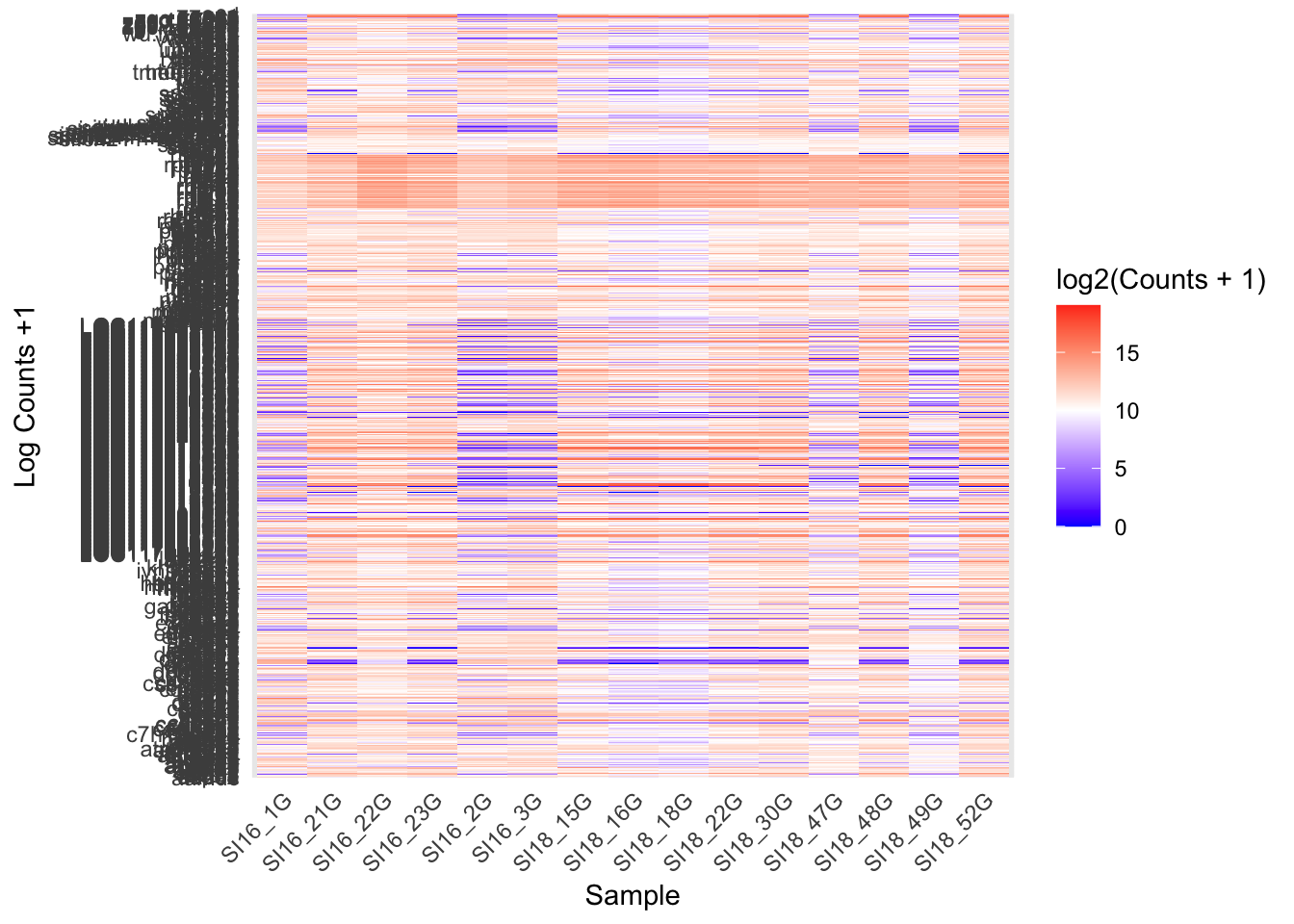
Genes are ordered alphabetically by default using ggplot, so there is preference to use different tools that cluster genes based on similar expression.
heatmap()
The heatmap() function from the base R stats package is another way to generate a heatmap, with clustering. It reorders genes using Euclidean distance to measure how similar their expression patterns are across samples, then repeatedly grouping the most similar genes together first. This builds a tree (the dendrogram shown alongside the heatmap), and reading gene order off that tree places genes with similar expression patterns next to each other. Genes that are co-expressed appear as visible blocks of colour.
my_colours1 <- colorRampPalette(c("blue", "white", "red"))(256)

heatmap(log2(as.matrix(counts_top1000) + 1),
        Rowv = TRUE,
        Colv = TRUE,
        labRow = NA,
        margins = c(8, 2),
        xlab = "Samples",
        ylab = "Gene",
        col = my_colours1)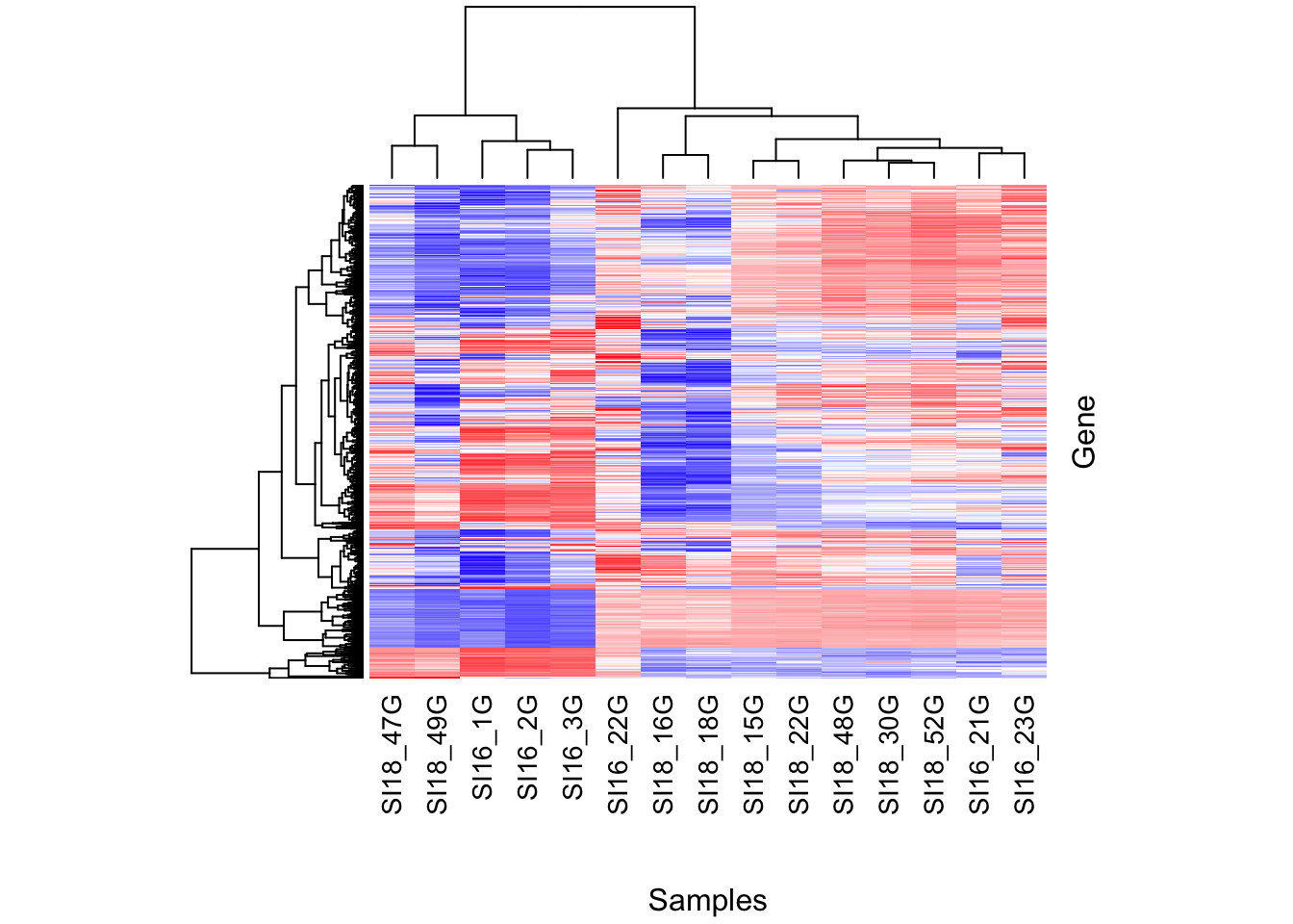
pheatmap()
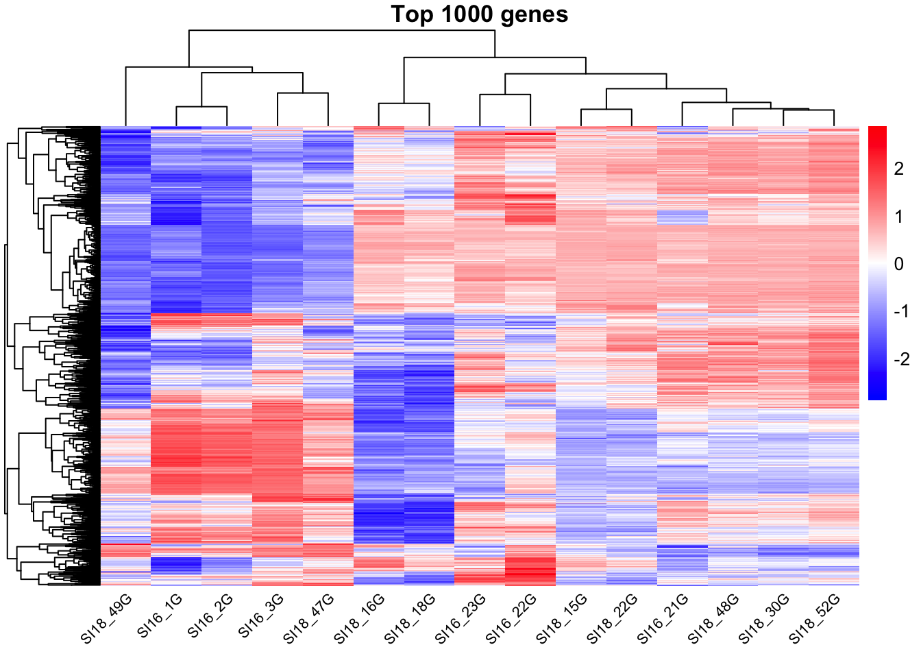
The pheatmap() function from the pheatmap package is another way to generate a heatmap, with clustering. It uses the same underlying clustering method as heatmap() by default, but is generally easier to customise.
scale = "row" z-scores each gene individually. For every gene, it subtracts the gene’s mean expression and divides by its standard deviation across samples. This means the heatmap shows each gene’s expression relative to its own average, rather than absolute expression level, so highly and lowly expressed genes can be compared on the same colour scale.
As with any plot, you will need to make visual adjustments (colour, breaks, scaling) based on your specific data and the range of values you are working with.
library(pheatmap)

pheatmap(log2(as.matrix(counts_top1000)+1),
         scale = "row", # Z-score normalisation across rows
         color = my_colours1,
         show_rownames = FALSE,
         cluster_rows = TRUE,
         cluster_cols = TRUE,
         angle_col = 45,
         fontsize_col = 8,
         main = "Top 1000 genes")