Introduction
Overview
Teaching: 10 min
Exercises: 0 minQuestions
What is genome assembly?
Objectives
Introduce the genome assembly workflow.
1.1 What is a reference genome assembly?
As genome sequencing and bioinformatic tools and technologies have rapidly developed in recent decades, we can now produce high-quality reference genome assemblies for species of interest. While a genome is the full complement of DNA characterising an individual organism and is inherent to all living beings, a reference genome is a tool used for research. A reference genome is the representative genome of a species. that can be used alone for interspecific comparisons or as a reference against which population-level resequencing or reduced-representation sequencing data can be aligned for high-quality variant calling for intra- or inter-specific comparisons. Further, reference genomes act as catalogues of gene coding sequences and other functional components, opening the door to a wide variety of biological applications.
Short reads vs. long reads
Short-read sequencing typically uses Illumina DNA sequencing platforms to produce reads with length <500 bp. Relatively small input DNA quantities are required, which makes short-read sequencing more accessible.
Long-read sequencing uses platforms such as Oxford Nanopore Technologies (ONT) or PacBio SMRT to produce reads with length >10,000 bp. Despite initial relatively low quality, ONT sequencing has experienced myriad improvements in wet-lab protocols, sequencing technology, and bioinformatic processing, resulting in sequencing data that is competitive with that of the more expensive high-quality PacBio HiFi data. Large amounts (micrograms) of high molecular weight intact DNA are required for these sequencing types. PacBio platforms are not yet available in Aotearoa, which may be a limiting factor for sequencing projects with taonga focal species.
While all genome assemblies are imperfect, reference genomes built purely from short-read data are prone to assembly errors due in part to the challenges associated with assembling long and complex repetitive sequences, or correctly assembling large structural variants. Such errors can result in incomplete genome assemblies, false variant detection, and incorrect gene annotation. Knowing these short-comings, long-read sequencing is now considered almost essential for producing high-quality genome assemblies.
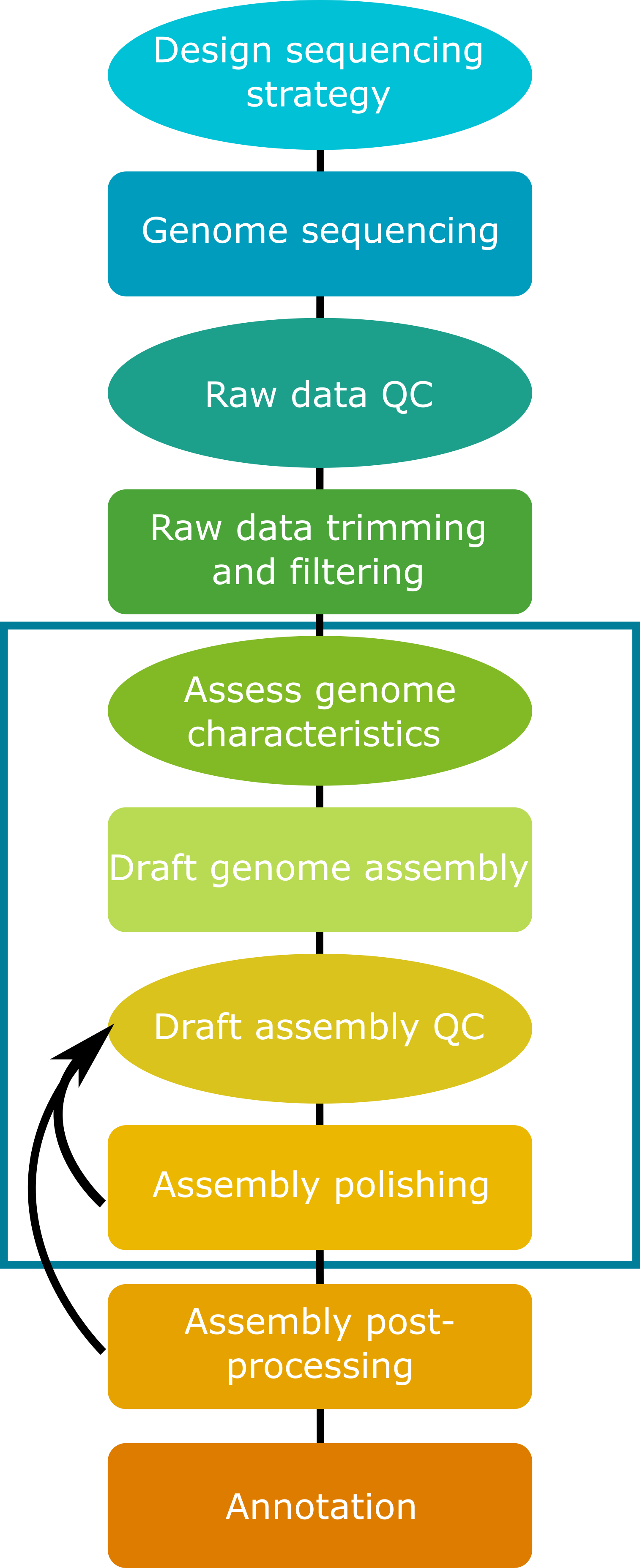
1.2 Steps in the genome assembly process
While genome assembly typically consists of a straightforward series of processes, it requires many choices at each step in the process. These choices include: sequencing type, sequence coverage depth, trimming and filtering parameters, genome assembly program, and downstream steps including polishing, scaffolding, and more. Many of these choices will be determined in part by the biological characteristics of the focal species and the target application(s) for the genome assembly.

Today we will assemble a small fungal genome using Oxford Nanopore Technologies long-read sequencing data in combination with Illumina short-read data. While we assemble this genome, we will consider the impacts of characteristics of the input data on each of the steps in the process.
An essential first step in working with sequencing data is raw read quality assessment, followed by appropriate trimming and filtering. For the purposes of today’s workshop, both long-read and short-read input data have been pre-processed through trimming and filtering steps to remove sequencing adapters and poor-quality sequences. Four subsets of data have been produced. We will work in groups to investigate the characteristics of these data sets, and the impacts of these characteristics on genome assembly quality at various stages of the pipeline.
This workshop has been designed to run on the NeSI compute infrastructure. All data and software has already been set up for you to use during the workshop.
Key Points
Understand the genome assembly workflow.
Using the slurm scheduler
Overview
Teaching: 10 min
Exercises: 10 minQuestions
How to submit jobs to an HPC scheduler
Objectives
Submit a job to the SLURM scheduler.
Derived from https://support.nesi.org.nz/hc/en-gb/articles/360000684396-Submitting-your-first-job
Shared resources and schedulers
The Mahuika HPC cluster provided by NeSI is a shared compute environment which means there needs to be a way of distributing resources in a fair way so that all users get the opportunity to use the cluster for their research needs. A complete list of resources can be found at Mahuika HPC Cluster resources but a summarised configuration is in the table below
| Node type | n | Cores/node | RAM/node |
|---|---|---|---|
| Login | 2 | 36 | 512GB |
| Compute | 226 | 36 | 128GB |
In order for the resources to be fairly managed, a scheduler is used to allocate resources. The login nodes allow for small interactive tasks to be done, but the bulk of the compute resource needs to be requested through the slurm scheduler which will take job resource requests, queue them, and distribute them throughout the compute nodes as suitable allocations become available.
On the Mahuika cluster, there are different ‘partitions’ or ‘queues’ depending on the resources being requested such as walltime, number of cpus, amount of ram, or gpu usage. This link has a list of the Mahuika Slurm Partitions.
Up until this point we have been using NeSI in an interactive manner, but we need to start requesting larger allocations of resources in order run our jobs in a timely manner.
The three main resources are:
- Number of CPUs,
- Memory (RAM), and
- Time (How long a job will be allowed to run for)
Creating a batch script
Jobs on Mahuika and Māui are submitted in the form of a batch script containing the code you want to run and a header of information needed by our job scheduler Slurm.
Create a new file and open it with nano myjob.sl
#!/bin/bash -e
#SBATCH --job-name=SerialJob # job name (shows up in the queue)
#SBATCH --time=00:01:00      # Walltime (HH:MM:SS)
#SBATCH --mem=512MB          # Memory in MB

pwd # Prints working directory
Copy in the above text and save and exit the text editor with ‘ctrl + x’.
Note:#!/bin/bash is expected by Slurm
Note: if you are a member of multiple accounts you should add the line #SBATCH --account=<projectcode>
Submitting a job
Jobs are submitted to the scheduler using:
sbatch myjob.sl
You should receive a similar output
Submitted batch job 1748836
sbatch can take command line arguments similar to those used in the shell script through SBATCH pragmas
You can find more details on its use on the Slurm Documentation
Using more CPUs
Often, bioformatics software has the option to use more CPUs or threads to make the processing go faster. In the case of SLURM, CPUs are a resource that need to be requested of if you are trying to use more than one.
Depending on the software, this is usually done using #SBATCH --cpus-per-task=N, where N is the number of CPUs you wish to use. You then can reference this number in your actual command using the variable SLURM_CPUS_PER_TASK. It’s a good idea to refer to this variable in your command so that if you increase or decrease the number of CPU cores from slurm this gets reflected in the command too. Usually bioinformatics programs that can make use of extra cpu cores will have a --threads or -t (or similar) argument.
#!/bin/bash -e
#SBATCH --job-name=SerialJob # job name (shows up in the queue)
#SBATCH --account=nesi02659  # account for the job
#SBATCH --time=00:01:00      # Walltime (HH:MM:SS)
#SBATCH --mem=512MB          # Memory in MB
#SBATCH --cpus-per-task=2    # Number of logical CPU cores being requested (2 logical cores = 1 physical core)

echo "Number of CPUs requested: $SLURM_CPUS_PER_TASK"
Job Queue
You can view all jobs that are currently in the job queue by using
squeue
If you want to see your jobs specifically you can use the -u flag and your username
squeue -u murray.cadzow
You can also filter to just your jobs using
squeue --me
You can find more details on its use on the Slurm Documentation
You can check all jobs submitted by you in the past day using:
sacct
Or since a specified date using:
sacct -S YYYY-MM-DD
Each job will show as multiple lines, one line for the parent job and then additional lines for each job step.
Cancelling
scancel <jobid> will cancel the job described by <jobid>. You can obtain the job ID by using sacct or squeue.
Tips
scancel -u [username] Kill all jobs submitted by you.
scancel {[n1]..[n2]} Kill all jobs with an id between [n1] and [n2]
Job Output
When the job completes, or in some cases earlier, two files will be added to the directory in which you were working when you submitted the job:
slurm-[jobid].out containing standard output.
slurm-[jobid].err containing standard error.
Job efficiency
As you run your jobs, it’s a good idea to keep efficiency in mind. You want to be requesting sufficient resources to complete your job, but not significantly more than you need “just in case” - the scheduler will assign all of the resource to you that you ask for regardless of if your task actually uses it all. The unused resource is unavailable to others to use so is wasted which is not ideal is a large, multi-user system like NeSI.
More is not always better. Requesting more CPU cores won’t always make things go faster - many programs don’t scale in a linear fashion, instead they have deminishing returns and will eventually hit a point where there is no increased performance.
We can determine the efficiency of our resource request usage through the nn_seff command. This will report back the job based on the resources requested and what was used.
The command is run like so: nn_seff <job_id>
Key Points
The SLURM scheduler faciliates the fair distribution of compute resource amongst users.
Exploring input data and genome characteristics
Overview
Teaching: 40 min
Exercises: 40 minQuestions
How do the characteristics of short-read and long-read datasets differ?
What underlying characteristics of a genome may complicate genome assembly?
Objectives
Build an understanding of how input data characteristics and underlying genome properties can impact genome assembly
3.1 Background and setup
It is getting easier and cheaper to sequence and assemble genomes. However, at the start of a genome project very little may be known about the genome properties of your organism of interest. Take genome size, for example. The amount and types of sequencing you would do, and the choice of assembly software will all be influenced by this parameter. There are 3 main approaches to obtaining a genome size estimate:
- If you are lucky to be working on a system where flow cytometry has been performed to quantify the amount of DNA (in picograms) in the nucleus of the cells of your organism, then you will have an estimate of genome size and ploidy to set alongside your draft sequence assembly. Such estimates are not always available, however.
- You might take a best guess, based on what is known about related taxa. In some cases this will be helpful. Birds, for example, display relatively little interspecific variation in genome size (typically 1.3 Gb, reported range from 1-2.1 Gb). In other cases, genome size can vary considerably: plant genome sizes range from 0.063 Gb (the carnivorous plant Genlisea) to 149 Gb (Paris japonica, in the Order Liliales) and often closely related taxa may have quite different genome sizes. Ploidy variation is also common and can have a major impact on genome size.
- Genome size can be estimated from unassembled and relatively low coverage short-read sequence data using k-mer profiles. We will explore this approach today.
This simple equation relates genome size to the amount of sequence data in an experiment and the coverage (which here means the average number of times that you have sequenced a base in the genome):
[G = \frac{T}{N}]
Where:
- G = genome size
- T = total bases sequenced
- N = genome coverage
Exercise
If you obtain 10 million read pairs (i.e. 2 x 100 bp reads) of whole genome sequence data for the plant Arabidopsis thaliana (genome size 120 Mb), what would the expected mean coverage be?
Solution
~16X
10,000,000 reads x 200 bp reads = 2,000,000,000 bp = T.
T / G = N
2,000,000,000 bp / 120,000,000 bp = 16.67X coverage.
Before we start, let’s move into the genome_assembly directory and consider what data has been provided for today’s workshop. First, take a look at the directory structure, what data has been provided, and make a new directory for results outputs. Using the ls -l command displays the files in a list, with additional information.
cd ~/obss_2022/genome_assembly/
ls
ls -l data/
mkdir results/
Exercise
What can you tell about the input data at first glance?
Solution
The input data is all in FASTQ format, which we have used previously in OBSS sessions.
There are two main data types: Illumina (short-read sequencing data) and ONT (Oxford Nanopore Technologies long-read sequencing data).
3.2 Input data quality assessment
Our raw data has been pre-processed, so let’s first get an overview of the quality and metrics of these processed data. For our Nanopore long-read data, there are specific tools that can assess quality and other metrics. One example is the program NanoStat.
As we saw earlier, we can use SLURM to submit scripts to the queue, which allows us to perform multiple processes simultaneously. Let’s navigate to the scripts directory and make a SLURM script to assess our Nanopore data.
cd ~/obss_2022/genome_assembly/scripts/
nano nanostat.sl
Copy the script below into the new file. Here you want to assess only the dataset that you are using in your assembly, so you will need to replace the * in the input and output filenames to one of A-E.
#!/bin/bash -e

#SBATCH --account=nesi02659
#SBATCH --job-name=nanostat
#SBATCH --output=%x.%j.out
#SBATCH --error=%x.%j.err
#SBATCH --time=15:00
#SBATCH --mem=1G

module purge
module load NanoStat

cd ~/obss_2022/genome_assembly/data/

# replace * with one of A-E
NanoStat --fastq all_trimmed_ont_*.fastq.gz -t1 > ~/obss_2022/genome_assembly/results/Nanostat_all_trimmed_ont_*
One benefit of using NeSI is that many commonly-used programs are pre-installed via modules. We use module purge to clear the module space before loading the modules we need for the job using the module load command.
Save the script and run it using sbatch nanostat.sl.
While NanoStat runs, we can use FastQC to assess the Illumina short read data in the same way that we used it yesterday.
module load FastQC

cd results/

fastqc ~/obss_2022/genome_assembly/data/All_trimmed_illumina.fastq.gz
Once FastQC has finished, check your queue to see whether NanoStat is still running, using squeue -u <nesi.id>. If it’s finished, use less to check your .err and .out logs in the scripts directory for any issues.
Now take a look at the results for FastQC and NanoStat, and discuss the overall metrics and quality with your neighbour. How do our short-read and long-read data sets differ from one another?
3.3 Genome size estimation and k-mer profiles
What are k-mers and k-mer profiles?
A k-mer is a substring of length k.
The maximum number of unique k-mers is given by 4k.
The numbers of k-mers contained within a sequence of length L is given by the equation L – K + 1, where L is the length of sequence and K is the k-mer length. A k-mer profile is a histogram in which the counts of the occurrences of each unique k-mer in the dataset are plotted. The x-axis shows the count of k-mer occurrence, often termed coverage or depth, and the y-axis the number of distinct k-mers which report that coverage/depth value.
Exercise
Consider the following 10bp sequence:
GTAGAGCTGT
Calculate how many 3-mers there are in this sequence using the equation L - K + 1. What are all the possible 3-mer sequences?
Solution
When L = 10 and K = 3:
L - K + 1 = 10 - 3 + 1 = 8.
There are 8 3-mers in the sequence:
GTA, TAG, AGA, GAG, AGC, GCT, CTG, TGT
K-mers have some convenient properties for computational biology: There are a finite number of distinct k-mers and the counting of these can be based on unambiguous matching. K-mer profiles for genome property estimation are usually 17-31 bases long. As k-mer length increases the likelihood of it occurring uniquely in your genome increases, but so does the chance that it will overlap a sequence error. Although 4k quickly becomes very large as k increases, the proportion of the total possible number of unique k-mers that are actually present in a genome decreases.
A typical k-mer profile
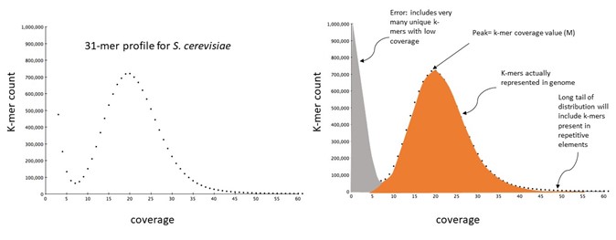
As we saw earlier, we can calculate G (genome size) using the equation G = T / N. However, at the outset of our analyses, we often only have a value for T.
We can obtain an estimate of the genome sequence coverage (N) by looking at the k-mer coverage, a property that can be calculated from unassembled reads in the following way:
[N = \frac{M * L}{L - K + 1}]
Where:
- N = genome sequence coverage
- M = the k-mer coverage (the peak of coverage on the k-mer profile plot)
- L = read length
- K = k-mer length
By estimating N in this way, we can combine it with our knowledge of T to obtain an estimate of G.
This approach to genome size estimation was proposed in the Giant Panda genome project, a landmark paper as it describes the first genome assembly to be generated from only short read Illumina sequencing (Li R, Fan W, Tian G, et al. 2010. The sequence and de novo assembly of the giant panda genome. Nature. doi:10.1038/nature08696).
We are going to use our processed Illumina short-read data to count k-mers that can be used to explore some characteristics of the sequenced genome, using a program called Jellyfish with our short-read data. Let’s navigate back to our scripts directory, and create a new script.
cd ../scripts/
nano jellyfish.sl
Copy the script below into your jellyfish.sl file.
#!/bin/bash -e
#SBATCH --job-name=jellyfish
#SBATCH --output=%x.%j.out
#SBATCH --error=%x.%j.err
#SBATCH --time=05:00
#SBATCH --mem=4G
#SBATCH --cpus-per-task=10
#SBATCH --account=nesi02659

module purge
module load Jellyfish/2.3.0-gimkl-2020a

cd ~/obss_2022/genome_assembly/results/

# decompress temporarily into a new file
gunzip -c ~/obss_2022/genome_assembly/data/All_trimmed_illumina.fastq.gz > ~/obss_2022/genome_assembly/data/All_trimmed_illumina.temp.fastq

# count 21-mers from read dataset
jellyfish count -C -m 21 -s 1G -t ${SLURM_CPUS_PER_TASK} -o kmer_21_illumina_reads.jf ~/obss_2022/genome_assembly/data/All_trimmed_illumina.temp.fastq

# remove temporary file
rm ~/obss_2022/genome_assembly/data/All_trimmed_illumina.temp.fastq

# generate histogram of kmer counts
jellyfish histo -t ${SLURM_CPUS_PER_TASK} kmer_21_illumina_reads.jf  > jf_reads.histo
Exercise
Question 1
First, let’s look at the SLURM resources. What can you tell about this job?
Now let’s examine how the script is navigating the directory structure. Where is the job being processed? Are any other paths included in this job?
Solution
The job will run for no more than 5 minutes, and will use up to 4 GB memory and 10 CPUs. We have given the job the name
jellyfishas an identifier. It will run under the account code for OBSS workshop.The job is being processed in the directory
~/obss_2022/genome_assembly/results/. The other path listed in the job is directing jellyfish to the input FASTQ data.Then let’s look at the commands we’ll be passing to Jellyfish. There are two steps to this process:
- Jellyfish counts the k-mers
- Jellyfish computes the histogram of these counts.
As you can see, there are a number of different parameters used, denoted by
-. A key part of bioinformatics is building familiarity with program manuals. These are often but not always hosted on GitHub, and provide information about program installation and usage.Question 2
If we know that Jellyfish is used to count k-mers, can you use Google to find the manual?
Solution
By googling ‘jellyfish genome k-mers’, you should be able to find the manual at https://github.com/gmarcais/Jellyfish.
Let’s save our jellyfish.sl file, and run it.
sbatch jellyfish.sl
We can check where our job is in the queue using squeue -u <nesi.id>. Then when the job finishes, we can check our log files to see if there are any problems or errors.
less jellyfish.*.out
less jellyfish.*.err
Check what outputs have been written to your results directory.
ls ../results/
To visualise the results of k-mer analysis, import your .histo file produced by Jellyfish into the GenomeScope webtool. Note: The input reads were produced from 150 bp Illumina sequencing.
What can you tell from these results, and how do your results compare to the examples at https://www.nature.com/articles/s41467-020-14998-3/figures/1?
3.4 Heterozygosity and k-mers
K-mer analyses can become more difficult in heterozygous diploid samples (and even more so for polyploids!). The challenge here is in correctly partitioning the k-mers that are derived from heterozygous and repetitive components of the genome. There are tools, such as GenomeScope, that model these different components of the profile and estimate genome properties.
The example below is for a pear genome. The profile left hand peak has a coverage of 0.5x the right hand peak. K-mers under the right peak are those sequences that are shared between both alleles at a locus, whereas sequence variants will change the identity of the k-mers that overlap these variants.

Exercise
The figure below is reproduced from Stevens et al. (2018; G3: Genes, Genomes, Genetics; 8:7, https://doi.org/10.1534/g3.118.200030). The authors present k-mer profiles for six different walnut (Juglans) species.
Key J. nigra Dashed blue P. stenoptera Solid blue J. sigillata Orange J. hindsii Green J. microcarpa Solid grey J. regia Dashed grey J. cathayensis Yellow Which of the species is (i) the most heterozygous and (ii) the least heterozygous?
Solution
i) P. stenoptera, ii) J. hindsii (based on the relative proportion in diploid vs haploid peaks).

Question 4: Which of the species is (i) the most heterozygous and (ii) the least heterozygous ?
Key Points
While long-read data are beneficial for producing high-quality genomes, short-read data can help understand the underlying properties of the genome of the focal species.
It is important to consider characteristics such as genome size, ploidy, and heterozygosity before assembling a genome, as this may influence program choice, parameter-setting, and overall assembly quality.
Draft genome assembly
Overview
Teaching: 10 min
Exercises: 10 minQuestions
What considerations should be taken into account when selecting a genome assembler?
Objectives
Assemble a small fungal genome.
4.1 Genome assembly options
A wide (and continually expanding) range of genome assembly tools are available. Many assemblers are designed for specific data types (e.g., short- vs long-reads, Nanopore vs PacBio data). It is important to select an assembler that is appropriate to the data type(s) and characteristics of the focal genome. Becoming familiar with genome assembly manuals and associated research can be helpful in understanding the strengths and weaknesses of the underlying algorithms implemented by the various assembly program.

4.2 Assembling a genome
Today we will be using Flye, an assembler designed to work with long-read data. Flye has modes for Nanopore and PacBio long-read data, that take into account the characteristics specific to each data type. We will use the --nano-raw mode to pass just our Nanopore data (labelled ‘ont’).
Although genome assembly algorithms are complex, using an assembler is typically very straightforward.
We will be making a series of scripts today to run different processes. Let’s set up our directory structure so we can keep things tidy. We will store all our scripts in the scripts directory. We also need to make a results directory to put the outputs we will generate.
cd ~/obss_2022/genome_assembly/
mkdir results/
cd scripts/
Using ls we can see that there are already some files in this directory. Take a look in your data directory to see what input data you have been given.
Now we will make our first script that will assemble a genome. To make a script, we will use a text editor called nano. Use the command nano flye.sl to open a new file called ‘flye.sh’ with nano. Now copy in the contents below:
#!/bin/bash -e

#SBATCH --job-name=FLYE
#SBATCH --account=nesi02659
#SBATCH --output=%x.%j.out
#SBATCH --error=%x.%j.err
#SBATCH --time=2:00:00
#SBATCH --mem=70G
#SBATCH --ntasks=1
#SBATCH --nodes=1
#SBATCH --cpus-per-task=32

module purge
module load Flye/2.9.1-gimkl-2022a-Python-3.10.5

# Change * to your group's dataset
flye --nano-raw ~/obss_2022/genome_assembly/data/all_trimmed_ont_*.fastq.gz --out-dir ~/obss_2022/genome_assembly/results/flye_raw_* -t ${SLURM_CPUS_PER_TASK}
You may have noticed that in our data/ directory, there is more than one .fastq.gz file. We are going to be working in groups today. The letter you are assigned corresponds to one of these data files, so you need to replace the two wildcards in the script above with the letter your group is assigned.
Now let’s save our new script and exit, using Ctrl+X. We have already named it flye.sh when we opened nano, so hit Y, and nano will save this and close. Check the contents of your scripts directory, and you should see this file.
As you can see from the SLURM resources, we expect this job to take around 2 hrs to run, so let’s check back later.
4.3 Later…

Now that we’ve got more familiar with looking at scripts in Section 3, let’s have a refresher on what the flye.sh script was doing. You should have an understanding of the SBATCH header now, but what about Flye itself? Let’s load the Flye module, and take a look at the help documentation to learn more about the program.
module load Flye/2.9.1-gimkl-2022a-Python-3.10.5

flye -h
Flye has really helpful help documentation! From this we can see that Flye can use both Nanopore and PacBio data to assemble a genome, but that we have to tell it what type of data we are giving it. Now let’s investigate the logs produced from running Flye.
Exercise
Look at your
.errand.outlogs for Flye. Were there any issues or errors? What can you tell about the process? What can you tell about the genome assembly?Solution
Take careful note of any ERROR messages. The logs describe the various processes implemented by Flye, and make some comments about the data along the way. At the end of the log there is a print-out of some brief assembly summary metrics, that will likely vary between groups.
After confirming that Flye ran correctly without any errors, we can investigate the outputs.
ls -lt ~/obss_2022/genome_assembly/results/flye_raw_*/
You should see a directory that looks like this:
  `-flye.log
  `-assembly_info.txt
  `-assembly.fasta
  `-assembly_graph.gfa
  `-assembly_graph.gv
  `-params.json
  |-40-polishing/
  |-30-contigger/
  |-20-repeat/
  |-10-consensus/
  |-00-assembly/
It is always important to check the log files for any other errors that may have occurred, or provide more details on resources used, or data characteristics. Flye logs contain very descriptive information about every step in the assembly process. This kind of transparent processing is valuable. You can see that a brief summary of these logs was printed to our .err file. If we jump to the end of the Flye log, we can see it prints the output directory contents, along with the brief summary of assembly statistics included in our .err file.
Most importantly, we can see there is a file called assembly.fasta. This contains the genome assembly produced by Flye in FASTA format. Let’s take a quick look at its contents.
head ~/obss_2022/genome_assembly/results/flye_raw_*/assembly.fasta
As expected for a FASTA file, we can see a header line denoted by > followed by a sequence line representing an assembled contig.
Congratulations, you’ve assembled a genome! But wait, there’s more…
Key Points
There are a wide variety of genome assembly programs available, each with specific strengths, weaknesses, and requirements. Building familiarity with a range of assemblers by reading program manuals and associated articles can be helpful.
Assessing assembly quality
Overview
Teaching: 20 min
Exercises: 30 minQuestions
How do we know whether a genome assembly is of sufficient quality to be biologically accurate?
Objectives
Explain key metrics used for assessing genome assembly quality.
Generate metrics for the genome assembly produced.
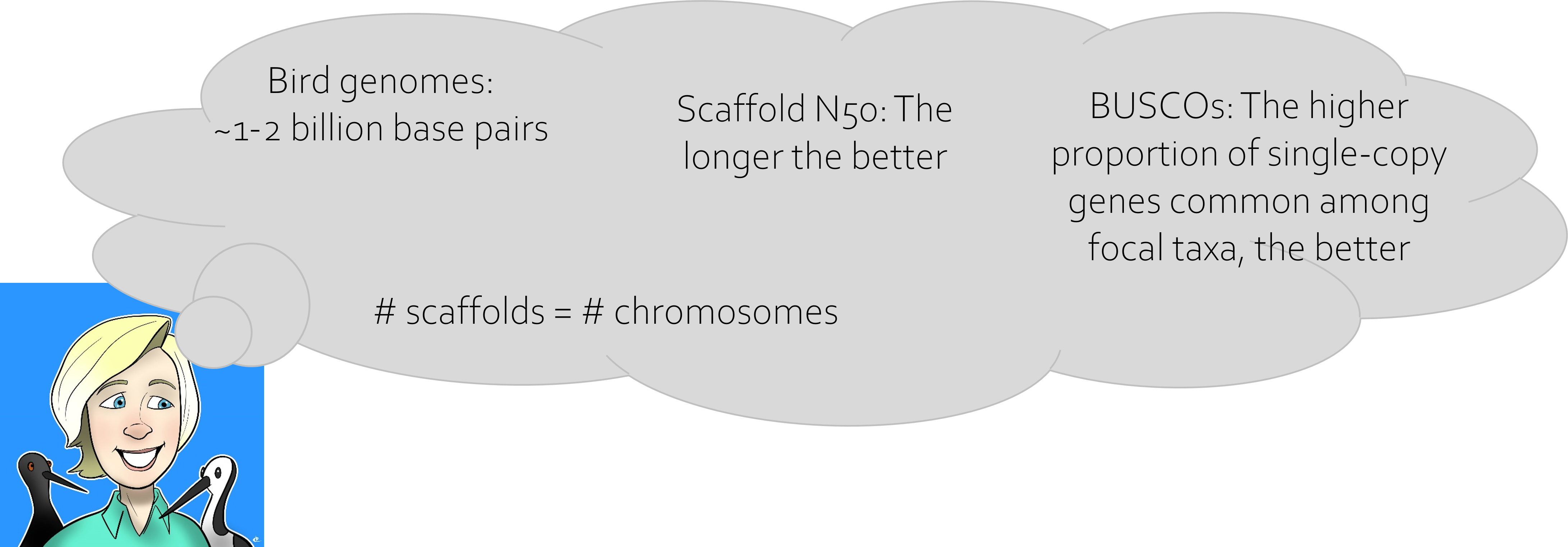
Assembly quality assessment
There are many factors to consider when assessing the quality of a genome assembly. Not only are we looking for an assembly that spans the expected genome size, but also we need to consider a range of other metrics.
In an ideal world, a genome assembly will span the expected genome size, be highly contiguous with one scaffold representing one chromosome and generally be comprised of long continuous scaffolds. The AT:GC ratio should be representative of that expected for the focal taxon. The assembly should contain the full set of expected gene orthologs (those genes common across species within a taxon). An ideal assembly will have consistent coverage across its length when the raw data is mapped gainst it, with no evidence of assembly errors. It will also contain only sequences from the focal organism, with no contaminating sequences from other species (e.g., no fungal sequences in a bird genome).
Even if an assembly is highly contiguous, or shows high completeness in terms of gene orthologs, there may be other issues that may not be identified using only those metrics. To investigate all of these aspects of an assembly requires a range of processes.
01. Basic metrics
An initial step in the assembly QC process is to generate basic assembly metrics. Today we will be using the assemblathon_stats.pl script to extract these metrics. You will need to modify the name of the input file depending on the read set you used for the assembly.
cd ~/obss_2022/genome_assembly/scripts/
./assemblathon_stats.pl ~/obss_2022/genome_assembly/results/flye_raw_*/assembly.fasta > ~/obss_2022/genome_assembly/results/flye_raw_assembly_QC.txt
Now let’s view the results.
less ~/obss_2022/genome_assembly/results/flye_raw_assembly_QC.txt
Exercise
Enter the metrics for your assembly into the shared spreadsheet. Are everyone’s results the same? If not, why may this be? How does your assembly compare to others?
Solution
We expect to see different results between groups based on the input data.
02. Gene orthologs
To assess assembly completeness in terms of the set of gene orthologs, we use a program called BUSCO. This identifies the presence of genes from a common database of gene common among the focal taxon (e.g., fungi) within the assembly. These genes are those that arose in a common ancestor and been passed on to descendant species. This means that selecting an appropriate database to make these comparisons is essential. For example, if I was assessing a bird genome, I would be best to select the ‘aves’ database rather than the ‘vertebrate’ database. Within an assembly, we expect these genes to be complete and present as a single copy.
#!/bin/bash -e

#SBATCH --job-name=busco
#SBATCH --account=nesi02659
#SBATCH --output=%x.%j.out
#SBATCH --error=%x.%j.err
#SBATCH --time=00:20:00
#SBATCH --mem=4G
#SBATCH --ntasks=1
#SBATCH --cpus-per-task=16

module purge
module load BUSCO/5.1.3-gimkl-2020a

cd ~/obss_2022/genome_assembly/results/

# Don't forget to correct the name of the input assembly directory
busco  -i flye_raw_*/assembly.fasta -c ${SLURM_CPUS_PER_TASK} -o flye_raw_assembly_busco -m genome -l fungi_odb10
Exercise
These results act as a proxy to tell us how ‘complete’ the assembly is.
Can you find the file containing a summary of the BUSCO results? Add the metrics for your assembly to the shared spreadsheet.
How do the results for your assembly differ from others? Why might this be?
Are everyone’s results the same? If not, why may this be? How does your assembly compare to that of other groups’?
Solution
We expect to see different results between groups based on the differences in input data.
03. Plotting coverage
Another form of evidence of assembly quality can come through plotting the sequence data back against the assembly. Spikes in coverage may indicate that repetitive regions have been collapsed by the assembler. On the other hand, regions of low coverage may indicate assembly errors that need to be corrected.
To investigate coverage, we will take our input Illumina data and map this to the genome assembly using bwa mem. We will then use bedtools to calculate mean coverage across genomic ‘windows’ - regions with a pre-determined size.
First, let’s make a new output directory for the results of this process.
mkdir ~/obss_2022/genome_assembly/results/coverage/
cd ~/obss_2022/genome_assembly/results/coverage/
We have quite a lot of short-read data compared with the data we used for mapping yesterday, so we will use a SLURM script for this step.
#!/bin/bash -e

#SBATCH --job-name=mapping
#SBATCH --account=nesi02659
#SBATCH --output=%x.%j.out
#SBATCH --error=%x.%j.err
#SBATCH --time=00:45:00
#SBATCH --mem=3G
#SBATCH --ntasks=1
#SBATCH --cpus-per-task=8

module purge
module load BWA/0.7.17-GCC-11.3.0 SAMtools/1.15.1-GCC-11.3.0

DATA=~/obss_2022/genome_assembly/data/
OUTDIR=~/obss_2022/genome_assembly/results/coverage/

cd ~/obss_2022/genome_assembly/results/flye_raw_*/

echo "making bwa index"
bwa index assembly.fasta

echo "mapping ONT reads"
bwa mem -t ${SLURM_CPUS_PER_TASK} assembly.fasta ${DATA}All_trimmed_illumina.fastq.gz | samtools view -S -b - > ${OUTDIR}mapped.bam

echo "sorting mapping output"
samtools sort -o ${OUTDIR}mapped.sorted.bam ${OUTDIR}mapped.bam

echo "getting depth"
samtools depth ${OUTDIR}mapped.sorted.bam > ${OUTDIR}coverage.out
While our data is mapping, we can prepare the genomic windows using BEDTools. First, let’s load the modules for the programs we need: BEDTools and SAMtools.
module load BEDTools/2.30.0-GCC-11.3.0
module load SAMtools/1.15.1-GCC-11.3.0
Now we want to gather information about the length of the contigs in the genome assembly. To do this, we can use SAMtools to index the genome. The index file produced contains the information we need to pass to BEDTools.
samtools faidx ~/obss_2022/genome_assembly/results/flye_raw_*/assembly.fasta
Now we will generate the genomic windows that we will calculate mean coverage across. We are going to set each window to 10 kb, making 5 kb steps before starting a new window.
bedtools makewindows -g ~/obss_2022/genome_assembly/results/flye_raw_*/assembly.fasta.fai -w 10000 -s 5000 > genomic_10kb_intervals.bed
Once our script has finished running, we can then continue the process to get the mean coverage across the genome assembly. First, let’s use head to see what information is in the final coverage.out file.
We will use awk to extract data from the coverage.out file produced by samtools depth and make the format readable by the BEDtools. awk is a widely used command line language that is really useful for manipulating files and extracting useful information. In the following command, we are producing a new file that will be in .bed format, containing 4 columns:
- the contig name
- the start position of the window within that contig
- the end position of the window within that contig
- the mean depth of coverage within that window
We tell awk to print the first column of coverage.out. It then inserts a tab space before printing the content of the second column. It inserts a tab again, before printing another column containing the sum of columns 1 and 2. Finally it adds another tab and then prints the third column of the coverage.out file.
awk '{print $1"\t"$2"\t"$2+1"\t"$3}' coverage.out > coverage.bed
Use head to compare the format and content of coverage.out and coverage.bed. Do you see what we did using awk?
We can then use BEDTools to do a function that calculates the mean coverage within each of the predefined windows. This makes it more efficient to plot coverage, as instead of plotting a point for every single base in the assembly, we will have one point (the mean depth) for every 10 kb window.
bedtools map -a genomic_10kb_intervals.bed -b coverage.bed -c 4 -o mean -g ~/obss_2022/genome_assembly/results/flye_raw_*/assembly.fasta.fai > 10kb_window_5kb_step_coverage.txt
Use head to check the format of this new output file, 10kb_window_5kb_step_coverage.txt.
Along with being a powerful tool for statistical analysis, R also is useful for data visualisation. We will then plot the mean coverage results file in RStudio. To do this, we need to open a new tab in Jupyter and select the RStudio launcher. Open a new Rscript file.
The first thing we need to do is to change our working directory to the directory where we have written all the coverage results.
setwd("~/obss_2022/genome_assembly/results/coverage/")
Next we want to pass the 10kb_window_5kb_step_coverage.txt file we just made in to R, ready to do some processing.
coverage <- read.delim("10kb_window_5kb_step_coverage.txt", header = FALSE)
We can use the R command head() in the same way that we use the bash command head to check the contents of the data file.
head(coverage)
Because we used header = FALSE when we read in the data file, you can see that R has automatically named our columns V1-V4. Let’s rename these to something more meaningful. To do this, we will use a package called reshape.
# load the reshape package
library(reshape)

# provide new column names
coverage<-rename(coverage,c(V1="contig", V2="startPos", V3="endPos",V4="meanDepth"))

# check the new headers
head(coverage)
To start with, we just want to look at the coverage across one contig. Each contig will have the same starting position (at 1), but the contigs are all different lengths. If we tried to plot the coverage for all the contigs in one plot, it would be messy and difficult to interpret.

Instead, we will do better to plot mean depth for each contig independently. Here we will just look at the first contig as an example, but you could choose the name of any contig in the genome assembly to investigate. To do this, we will use a package called dplyr that can help us filter our dataset.
First let’s find out what the names of all the contigs are in the genome assembly. NOTE: Assemblies produced using different datasets may have different numbers of contigs, and the contigs may have different names.
unique(coverage$contig)
Now we know the contig name, we can extract the data for just that contig.
# load the dplyr package
library(dplyr)

# From the coverage dataset, we will make a new object called 'contig_10' that only contains the data for contig_10
contig_10 <- coverage %>%
  filter(contig == "contig_10")
Now we are ready to create a coverage plot. To make the most basic plot in R we can use the plot command.
plot(contig_10$startPos, contig_10$meanDepth, type = "l")
Can you identify any regions with very high or very low coverage compared to the overall pattern across the contig? What may have caused this?
04. Summary
So now we have an idea of our assembly characteristics. It can be useful to compare these metrics against those for other closely related taxa in the published literature. Like genome size, there may be some genome characteristics that are inherent to a taxon. For example, birds have highly conserved genomes, so we expect all bird genome assemblies to be around 1-1.5 Gb, and to see a particular skew to the AT:GC ratios.
It is very useful to generate these metrics after each step in downstream genome assembly processing, so we can identify the extent of the improvements we are making to the genome. We will expect to see diminishing improvements as we progress.
Key Points
All genome assemblies are imperfect, but some are more imperfect than others. The quality of an assembly must be assessed using multiple lines of evidence.
Assembly polishing and post-processing
Overview
Teaching: 20 min
Exercises: 40 minQuestions
How can we improve a draft assembly to make it more correct and accurate?
Objectives
Polish draft genome assembly using Nanopore long-reads and Illumina short-reads to correct errors.
The genome assembly produced at this stage is still in draft form, and there are several ways we can make improvements to it. It is good practice to compare assembly metrics at the end of each step in these processes to see whether the assembly is continuing to improve. The first step for assemblies produced with Nanopore data is assembly polishing.
6.1 Long-read polishing
Nanopore data is really useful for genome assembly due to the length of the reads produced, meaning it is easier to piece the genome together into contiguous scaffolds. However, Nanopore data has a higher rate of sequencing error than other data types like Illumina or PacBio HiFi. Polishing is a process where reads are mapped against the assembly to identify errors which can then be corrected using the consensus of the mapped data.
We will first perform polishing using the Nanopore data itself, using the program Medaka. Let’s make a script for Medaka using nano medaka.sl.
#!/bin/bash -e

#SBATCH --job-name=medaka
#SBATCH --account=nesi02659
#SBATCH --output=%x.%j.out
#SBATCH --error=%x.%j.err
#SBATCH --time=00:18:00
#SBATCH --mem=12G
#SBATCH --ntasks=1
#SBATCH --cpus-per-task=4
#SBATCH --gpus-per-node A100:1

module purge
module load medaka/1.6.0-Miniconda3-4.12.0

cd ~/obss_2022/genome_assembly/results/

medaka_consensus -i ~/obss_2022/genome_assembly/data/all_trimmed_ont_*.fastq.gz -d flye_raw_*/assembly.fasta -o medaka_polish  -t ${SLURM_CPUS_PER_TASK} -m r941_min_sup_g507
It is good practice to compare assembly metrics at the end of each step in these processes to see whether the assembly is continuing to improve. In the interests of time, today we will just use our assemblathon_stats.pl script to collect metrics, and run BUSCO once more at the end of our polishing steps.
6.2 Short-read polishing
After polishing the assembly with the Nanopore long reads, we can also leverage the high-quality Illumina short read data to perform additional polishing. We will do this with Pilon. To run Pilon we need both the assembly FASTA file, and a BAM file of the short reads mapped to the assembly. You can read more about the various parameters in the Pilon usage guide. To make the BAM file, create a new script called make_bam.sl, and copy in the script below.
#!/bin/bash -e

#SBATCH --job-name=samtools
#SBATCH --account=nesi02659
#SBATCH --output=%x.%j.out
#SBATCH --error=%x.%j.err
#SBATCH --time=40:00
#SBATCH --mem=8G
#SBATCH --ntasks=1
#SBATCH --cpus-per-task=4

module purge
module load BWA SAMtools

cd ~/obss_2022/genome_assembly/results/medaka_polish/

# step 1. index assembly
bwa index consensus.fasta

cd ~/obss_2022/genome_assembly/results/

# step 2. map short reads
bwa mem medaka_polish/consensus.fasta ~/obss_2022/genome_assembly/data/All_trimmed_illumina.fastq.gz > illumina_trimmed_mapped_to_medaka_consensus.sam

# step 3. sort mapped reads
samtools sort  -@ ${SLURM_CPUS_PER_TASK} -o illumina_trimmed_mapped_to_medaka_consensus.sorted.bam illumina_trimmed_mapped_to_medaka_consensus.sam

# step 4. make index of sorted mapped reads
samtools index illumina_trimmed_mapped_to_medaka_consensus.sorted.bam
There are four steps in this process that use the programs BWA and SAMtools:
bwa indexcreates an index of the assembly so it can be read bybwa membwa memis used to map the Illumina reads to the Medaka polished assemblysamtools sortsorts the mapped reads by coordinate (their location in the assembly)samtools indexcreates an index of the sorted mapped reads for rapid access by Pilon
While this runs, we can prepare the script for Pilon polishing. Make a new file called pilon.sl, and copy the following script into it.
#!/bin/bash -e

#SBATCH --job-name=pilon
#SBATCH --account=nesi02659
#SBATCH --output=%x.%j.pilon.out
#SBATCH --error=%x.%j.pilon.err
#SBATCH --time=20:00
#SBATCH --mem=18G
#SBATCH --ntasks=1
#SBATCH --cpus-per-task=16

module purge
module load  Pilon/1.24-Java-15.0.2

cd ~/obss_2022/genome_assembly/results/

java -Xmx16G -jar $EBROOTPILON/pilon.jar \
    --genome medaka_polish/consensus.fasta \
    --frags illumina_trimmed_mapped_to_medaka_consensus.sorted.bam \
    --changes --vcf --diploid --threads ${SLURM_CPUS_PER_TASK} \
    --output medaka_pilon_polish1 \
    --minmq 30 \
    --minqual 30
Use assemblathon_stats.pl to investigate how polishing has impacted the basic assembly metrics. We can also modify our BUSCO.sl script to compare the gene completeness of this polished version of the assembly with our original draft. To do this, change the input directory and assembly filename to the Pilon output, and change the BUSCO output filename.
For both long- and short-read polishing, you may find a genome assembly can benefit from multiple rounds of polishing, with continued improvements in the assembly metrics.
6.3 Downstream processes
Today we have produced a fungal draft genome assembly. You can see that there are a number of steps in the process, and that many choices must be made along the way, based on input data types, genome characteristics of the focal organism, and the quality of the assembly produced.
While we’ve done a lot of work to get to produce this draft assembly, there is still more that can be done before a genome is published or used for downstream research. Take a look at the detailed workflow below. Which steps did we complete today? How many more steps could we work through? A lot of work goes into producing a high-quality genome assembly!

Key Points
Multiple rounds of polishing using different data sets can improve the accuracy of a genome assembly, and is particularly important when assemblies are produced using Nanopore data.
We have done a lot of work to get our genome assembly to this stage, but there are a number of downstream processes that can be done that can further improve the assembly and make it more useful for biological research.